library(crypto)
library(RGENERATE)
library(quantmod)
library(lubridate)
library(tseries)
library(tidyverse)
library(forecast)

times <- RGENERATE::generate(FUN = rnorm, n = 1000, K = 3,names = c("asset1")) %>%
  mutate(price = cumsum(asset1)+300) %>%
  mutate(day = row_number())

times %>%
  ggplot(aes(day, price))+
  geom_line()+theme_minimal() +
  geom_smooth(method = 'lm', lty = 2, colour = 'red', se = F)+
  labs(title = "Dynamically created time series",
       subtitle = "Created using the RGENERATE pakage")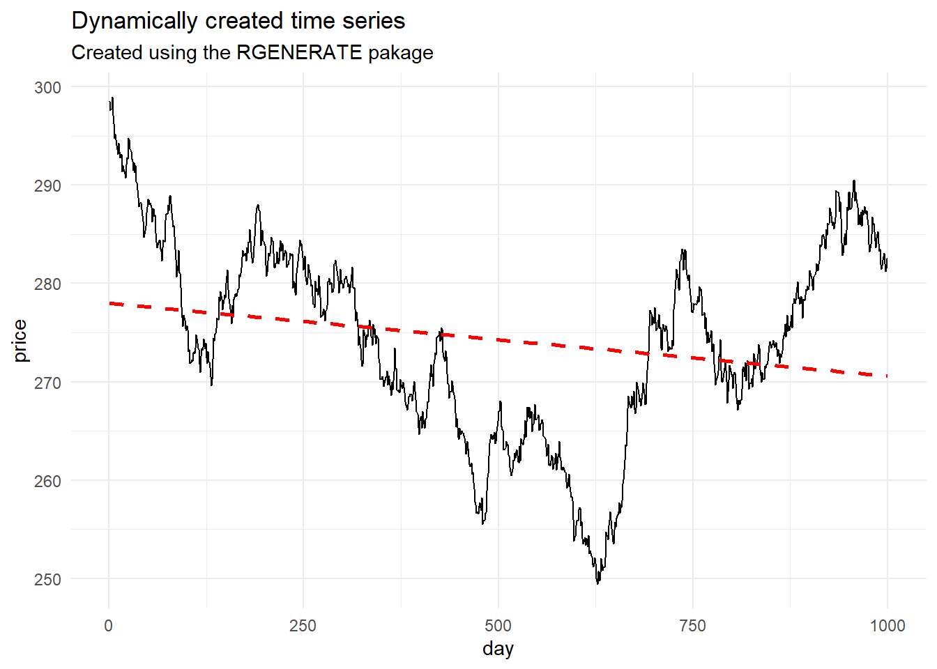
ARIMA modelling assumptions
\[X_t = c + \epsilon_t + \sum_{i=1}^p\beta_iX_{t-i}+\sum_{i=1}^q\theta_i\epsilon_{t-i}\]
An ARIMA model is a regression combining an autoregression with integration and a moving average.
For example, an ARIMA(3, 2, 5) model refers to a model with 3 autoregressive terms like \(X_t = \beta_1X_{t-1}+\ldots+\beta_3X_{t-3}+\ldots\), 2 orders of differencing to remove non-stationarity, and 5 moving average terms \(X_t=\ldots+\theta_{1} \epsilon_{t-1}+\ldots+\theta_5\epsilon_{t-5}\)
We should be able to test to see which is the optimal number of terms to use for our model to aid in predictive power.
The ARIMA model assumes that the data is univariate, that is it assumes there is only one explanatory variable, that being the previous consecutive price point.
It also assumes the data to be stationary, that is the error term \(\epsilon_t\) is normally distributed and considered to be ‘white-noise’.
Augmented Dickey-Fuller test
The Dickey-Fuller test checks to see if the time series is stationary. It is possible to simply plot the residuals of the data and then ‘eyeball’ it to see if the error terms largely tend towards zero and are normally distributed, that is \(\epsilon_t\) ~ \(\\N(0, \sigma^2)\). Otherwise…
\[\Delta y_t=c+\beta t + \gamma y_{t-1} + \sum_{i = 1}^{p}\delta\Delta y_{t-i} + e_t\] where \(c =\) regression constant. \(\beta\), \(\gamma\), \(\delta_i\) are regression coefficients. \(p =\) number of lagged terms. The Dickey-Fuller test tests for significance of the \(\gamma\) coefficient with the null hypothesis \(H_0 : \gamma = 1\), meaning that the lag coefficient is significant therefore the time series is non-stationary against \(H_1:\gamma \neq1\), meaning that the lag variable coefficient is insignificant and that the model exhibits stationarity.
(adf_output <- adf.test(times$price))##
## Augmented Dickey-Fuller Test
##
## data: times$price
## Dickey-Fuller = -1.8879, Lag order = 9, p-value = 0.6258
## alternative hypothesis: stationaryadf_output$p.value## [1] 0.6257587adf_output$significant <- ifelse(adf_output$p.value<0.05,"significant","insignificant")The p value of 0.63 is insignificant which allows us to infer that our time series data exhibits non-stationarity as the lag variable has a significant coefficient. We are unable to reject the null hypothesis that the coefficient is equal to 1.
In the case of non-stationarity, there are a few options to coerce stationarity such as taking the log or the square roots of the data to stabalise non-constant variance, calculating the residuals from another fitted model, or simply taking another difference of our series data, that is \(\Delta^2\).
This can be demonstrated as follows
times <- times %>%
  mutate(diff_price = price - lag(price)) %>%
  filter(!is.na(diff_price))

times %>% ggplot(aes(day, diff_price)) + geom_line()+
  geom_smooth(method = 'lm', lty = 2, colour = 'red', se = F)+
  theme_void()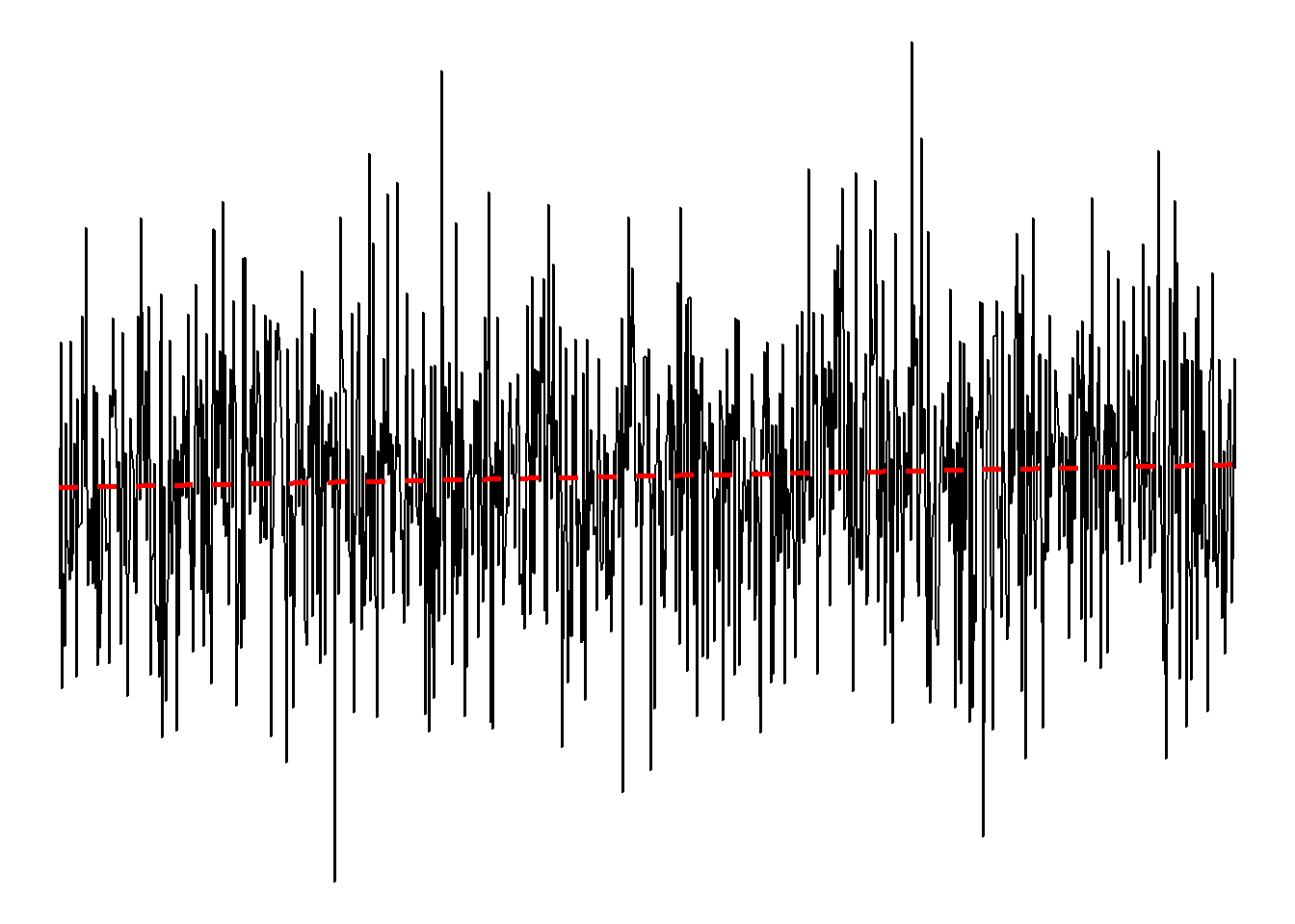
ts(times$diff_price, start = c(2000,1), frequency = 365) %>%
  decompose()%>%
  plot()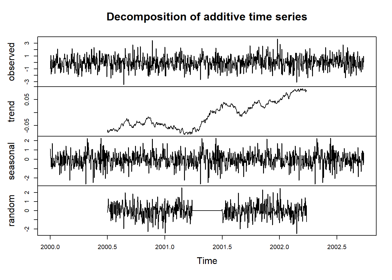
adf.test(times$diff_price)##
## Augmented Dickey-Fuller Test
##
## data: times$diff_price
## Dickey-Fuller = -9.8596, Lag order = 9, p-value = 0.01
## alternative hypothesis: stationaryMany other unit root tests exist such as the Kwiatkowski-Phillips-Schmidt-Shin (KPSS) test.
Alternatively, seasonality can be removed from the time series data using the in-built R stats functions.
times.decomposed <- ts(times$price, start = c(2000,1), frequency = 365) %>%
  decompose()
times.season.adj <- times$price - times.decomposed$seasonal

times.season.adj.test <- diff(times.season.adj, differences = 1)

plot(times.season.adj.test)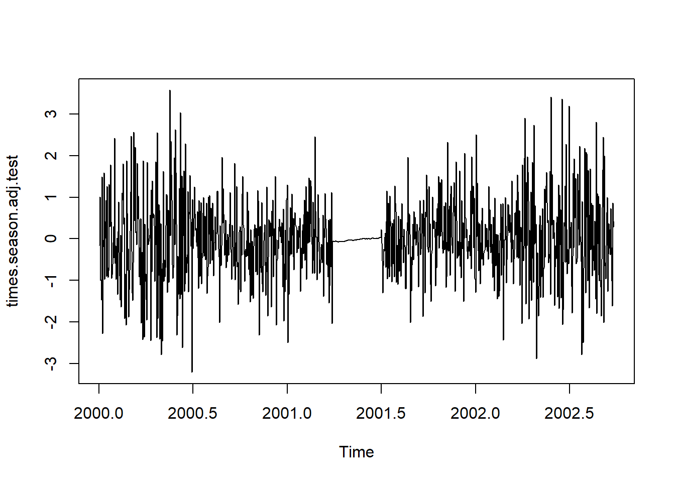
Fitting the model
There are options to choose from for how we estimate the accuracy of our model. Namely, ML = Maximum Likelihood estimation, AIC = Akaike Information Criterion,
acf(times$price, lag.max=70)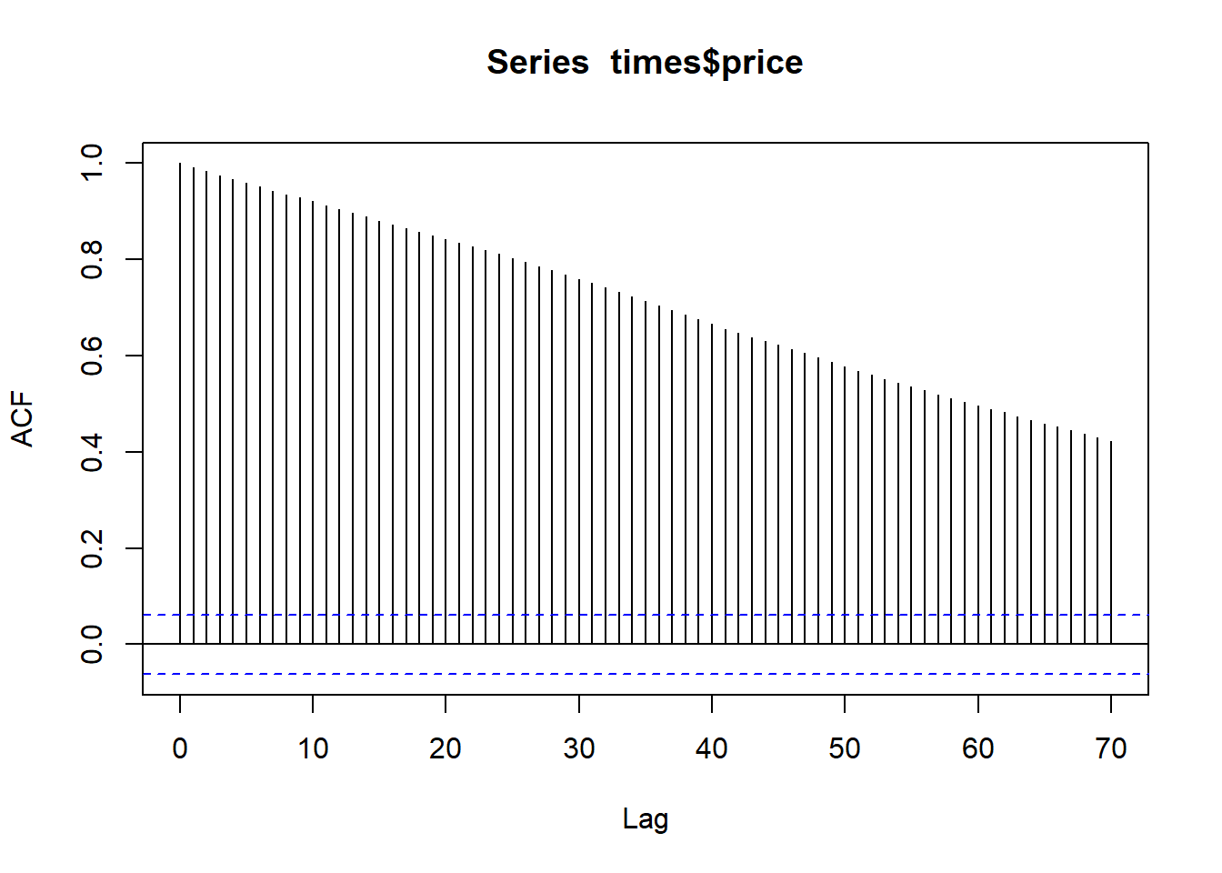
fitARIMA <- arima(times$price, order=c(1,1,1),seasonal = list(order = c(1,0,0), period = 12),method="ML")


confint(fitARIMA)
## 2.5 % 97.5 %
## ar1 NaN NaN
## ma1 NaN NaN
## sar1 -0.01910548 0.1051607Instead of going through each iteration of Arima(x, y, z) and selecting the best model, we can use the auto.arima() function in R from the forecasts package.
times.arima_auto_model <- auto.arima(times$price %>% log(), trace = TRUE)##
## Fitting models using approximations to speed things up...
##
## ARIMA(2,1,2) with drift : -8324.657
## ARIMA(0,1,0) with drift : -8328.556
## ARIMA(1,1,0) with drift : -8325.609
## ARIMA(0,1,1) with drift : -8326.561
## ARIMA(0,1,0) : -8330.367
## ARIMA(1,1,1) with drift : -8323.594
##
## Now re-fitting the best model(s) without approximations...
##
## ARIMA(0,1,0) : -8341.565
##
## Best model: ARIMA(0,1,0)Forecasting with the Arima model
times.predictions <- forecast::forecast(object = times$price %>% log(), model = times.arima_auto_model, h = 30)


times.predictions %>% plot()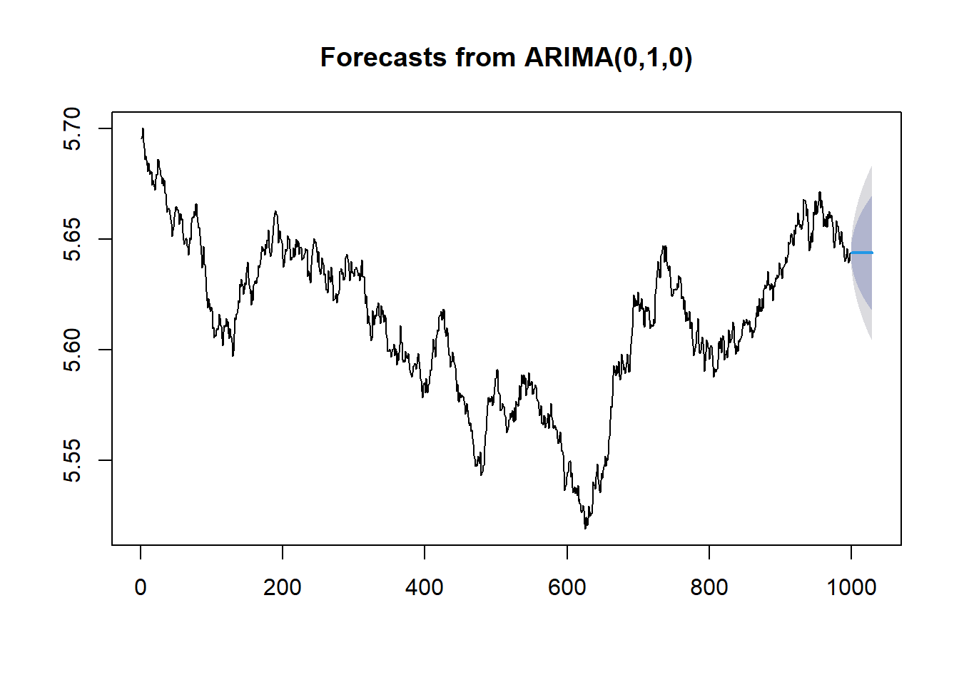
times.predictions <- as.tibble(times.predictions)


cbind(times.predictions, day = 1:nrow(times.predictions)+999) %>%
  ggplot(aes(day, times.predictions$`Point Forecast`))+
  geom_ribbon(aes(ymin = `Lo 95`, ymax = `Hi 95`), alpha = 0.2, colour = "black", fill = "dodgerblue")+
  geom_ribbon(aes(ymin = `Lo 80`, ymax = `Hi 80`), alpha = 0.2, colour = "black", fill = "blue")+
  theme_minimal()+
  geom_line(lty = 2)+
  labs(title = "Forecasting asset price with the Arima model",
       subtitle = "A 60 day forecast - 95% and 80% confidence intervals",
       y = "price")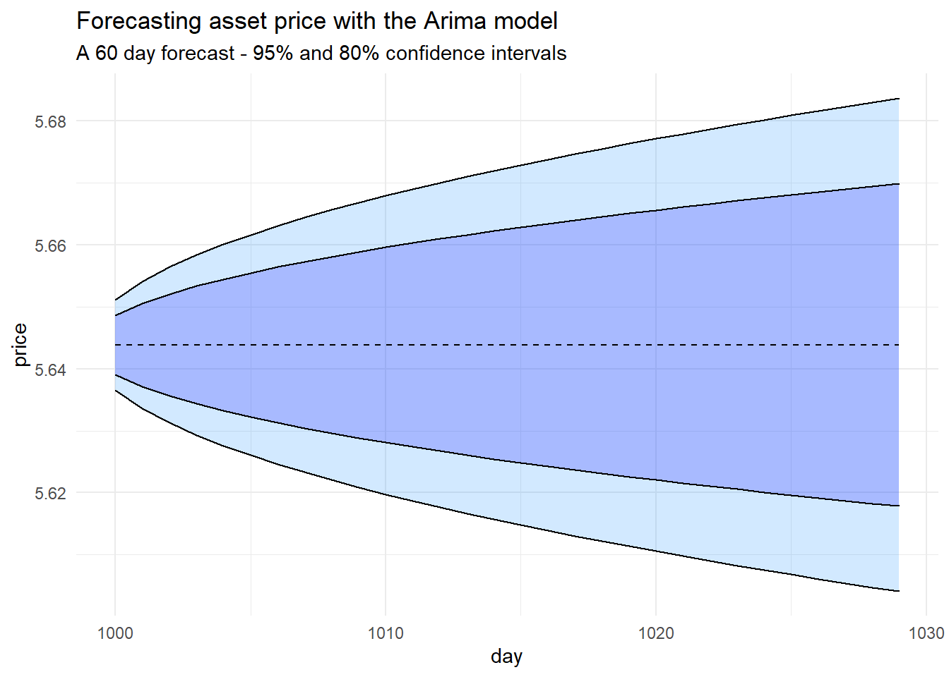
Forecasting real-world price data
Tesla
#btc <- read_csv("btc.csv")

quantmod::getSymbols("TSLA")
## [1] "TSLA"tsla_model <- log(TSLA$TSLA.Close) %>% auto.arima(trace = TRUE, stationary = FALSE)##
## Fitting models using approximations to speed things up...
##
## ARIMA(2,1,2) with drift : -10588.87
## ARIMA(0,1,0) with drift : -10559.17
## ARIMA(1,1,0) with drift : -10556.19
## ARIMA(0,1,1) with drift : -10557.18
## ARIMA(0,1,0) : -10554.44
## ARIMA(1,1,2) with drift : Inf
## ARIMA(2,1,1) with drift : -10572.54
## ARIMA(3,1,2) with drift : -10588.01
## ARIMA(2,1,3) with drift : -10588.29
## ARIMA(1,1,1) with drift : Inf
## ARIMA(1,1,3) with drift : -10550.88
## ARIMA(3,1,1) with drift : -10581.34
## ARIMA(3,1,3) with drift : Inf
## ARIMA(2,1,2) : -10582.86
##
## Now re-fitting the best model(s) without approximations...
##
## ARIMA(2,1,2) with drift : -10562.93
##
## Best model: ARIMA(2,1,2) with drifttsla_forecast <- forecast::forecast(object = TSLA$TSLA.Close, model = tsla_model, h = 60)
forecast(tsla_model, h = 70) %>% plot()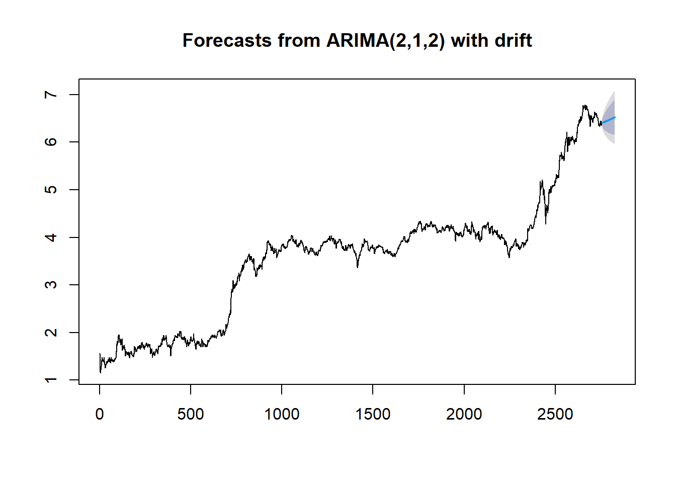
Amazon
quantmod::getSymbols("AMZN")## [1] "AMZN"AMZN_model <- log(AMZN$AMZN.Close) %>% auto.arima(trace = TRUE, stationary = FALSE)##
## Fitting models using approximations to speed things up...
##
## ARIMA(2,1,2) with drift : -16841.78
## ARIMA(0,1,0) with drift : -16839.48
## ARIMA(1,1,0) with drift : -16839.27
## ARIMA(0,1,1) with drift : -16840.53
## ARIMA(0,1,0) : -16831.92
## ARIMA(1,1,2) with drift : -16844.08
## ARIMA(0,1,2) with drift : -16847.08
## ARIMA(0,1,3) with drift : -16845.07
## ARIMA(1,1,1) with drift : -16842.87
## ARIMA(1,1,3) with drift : Inf
## ARIMA(0,1,2) : -16837.88
##
## Now re-fitting the best model(s) without approximations...
##
## ARIMA(0,1,2) with drift : -16854.55
##
## Best model: ARIMA(0,1,2) with driftAMZN_forecast <- forecast::forecast(object = AMZN$AMZN.Close, model = AMZN_model, h = 70)
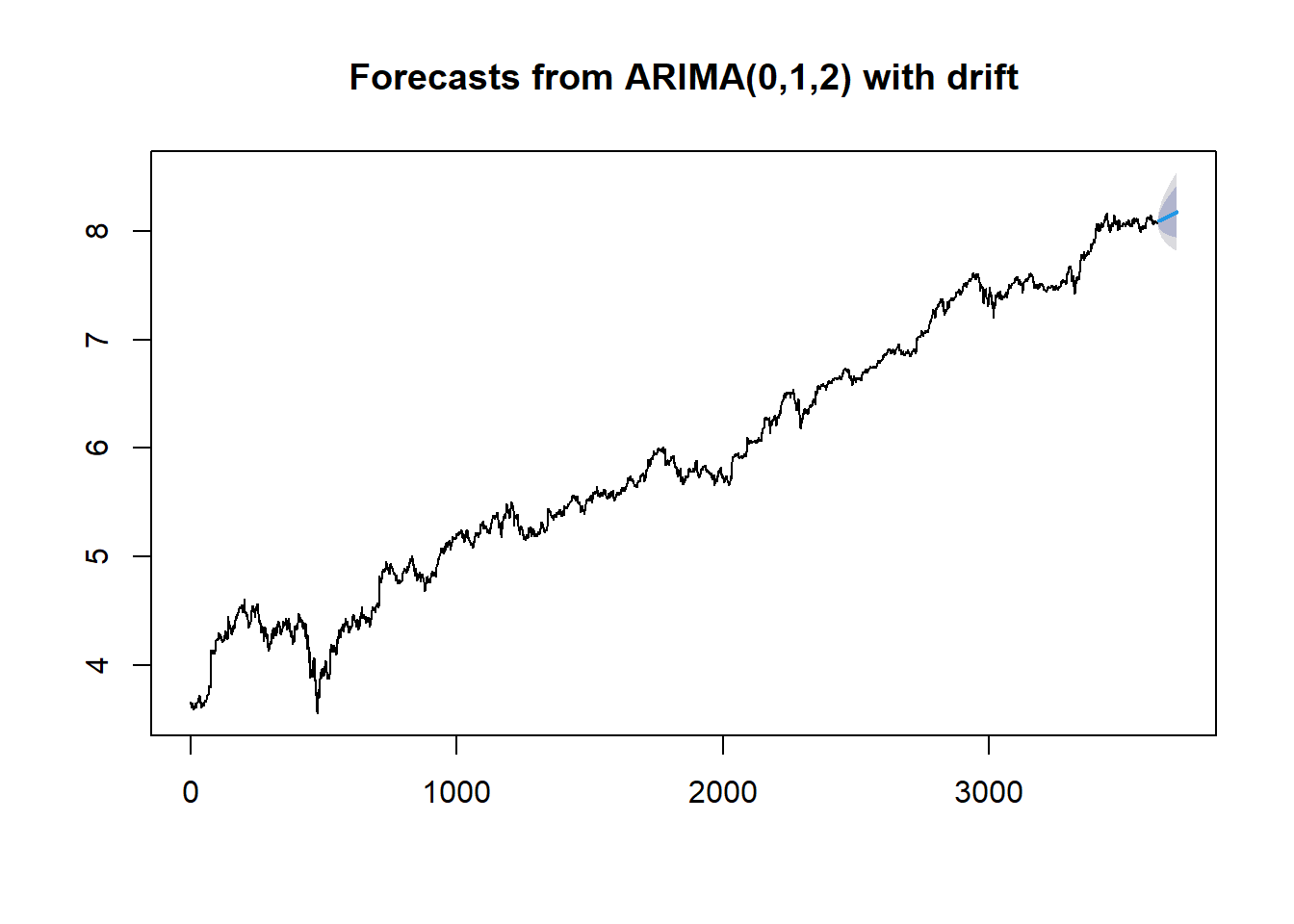
forecast(AMZN_model, h = 70) %>% plot()