library(tidyverse)
library(readr)
library(broom)
theme_set(theme_minimal())

heart <- read_csv("heart.csv")
The dataset can be found on kaggle
glimpse(heart)## Rows: 303
## Columns: 14
## $ age <dbl> 63, 37, 41, 56, 57, 57, 56, 44, 52, 57, 54, 48, 49, 64, 58, 5~
## $ sex <dbl> 1, 1, 0, 1, 0, 1, 0, 1, 1, 1, 1, 0, 1, 1, 0, 0, 0, 0, 1, 0, 1~
## $ cp <dbl> 3, 2, 1, 1, 0, 0, 1, 1, 2, 2, 0, 2, 1, 3, 3, 2, 2, 3, 0, 3, 0~
## $ trtbps <dbl> 145, 130, 130, 120, 120, 140, 140, 120, 172, 150, 140, 130, 1~
## $ chol <dbl> 233, 250, 204, 236, 354, 192, 294, 263, 199, 168, 239, 275, 2~
## $ fbs <dbl> 1, 0, 0, 0, 0, 0, 0, 0, 1, 0, 0, 0, 0, 0, 1, 0, 0, 0, 0, 0, 0~
## $ restecg <dbl> 0, 1, 0, 1, 1, 1, 0, 1, 1, 1, 1, 1, 1, 0, 0, 1, 1, 1, 1, 1, 1~
## $ thalachh <dbl> 150, 187, 172, 178, 163, 148, 153, 173, 162, 174, 160, 139, 1~
## $ exng <dbl> 0, 0, 0, 0, 1, 0, 0, 0, 0, 0, 0, 0, 0, 1, 0, 0, 0, 0, 0, 0, 0~
## $ oldpeak <dbl> 2.3, 3.5, 1.4, 0.8, 0.6, 0.4, 1.3, 0.0, 0.5, 1.6, 1.2, 0.2, 0~
## $ slp <dbl> 0, 0, 2, 2, 2, 1, 1, 2, 2, 2, 2, 2, 2, 1, 2, 1, 2, 0, 2, 2, 1~
## $ caa <dbl> 0, 0, 0, 0, 0, 0, 0, 0, 0, 0, 0, 0, 0, 0, 0, 0, 0, 0, 0, 2, 0~
## $ thall <dbl> 1, 2, 2, 2, 2, 1, 2, 3, 3, 2, 2, 2, 2, 2, 2, 2, 2, 2, 2, 2, 3~
## $ output <dbl> 1, 1, 1, 1, 1, 1, 1, 1, 1, 1, 1, 1, 1, 1, 1, 1, 1, 1, 1, 1, 1~N = 303
Explanation of features
- age - age in years
- sex - sex (1 = male; 0 = female)
- cp - chest pain type (1 = typical angina; 2 = atypical angina; 3 = non-anginal pain; 0 = asymptomatic)
- trestbps - resting blood pressure (in mm Hg on admission to the hospital)
- chol - serum cholestoral in mg/dl
- fbs - fasting blood sugar > 120 mg/dl (1 = true; 0 = false)
- restecg - resting electrocardiographic results (1 = normal; 2 = having ST-T wave abnormality; 0 = hypertrophy)
- thalach - maximum heart rate achieved
- exang - exercise induced angina (1 = yes; 0 = no)
- oldpeak - ST depression induced by exercise relative to rest
- slope - the slope of the peak exercise ST segment (2 = upsloping; 1 = flat; 0 = downsloping)
- ca - number of major vessels (0-3) colored by flourosopy
- thal - 2 = normal; 1 = fixed defect; 3 = reversable defect
- output - diagnosis of heart disease
It is my understanding that the ST is a specific interval of time during an electrocardiogram stress test.
Exploring the dataset
heart %>%
  count(output)
## # A tibble: 2 x 2
## output n
## <dbl> <int>
## 1 0 138
## 2 1 165The dataset represents 54.46% of people who suffer with heart disease.
Variance-covariance matrix and correlation matrix
g <- cor(heart)

h <- reshape2::melt(cov(heart))

ggplot(h, aes(Var1, Var2)) + geom_tile(aes(fill = log(abs(value)))) +
  ggtitle("Variance-covariance matrix")+
  labs(x="",y="")+
  theme(axis.text.x = element_text(angle = 90))+
  geom_text(aes(x = Var1, y= Var2,label = round(value,2)),size = 2)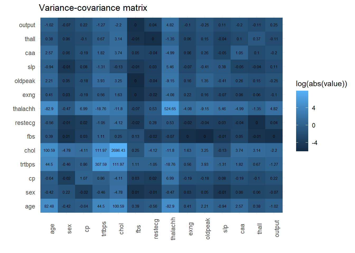
cov(g) %>%
  heatmap()
corrplot::corrplot(g)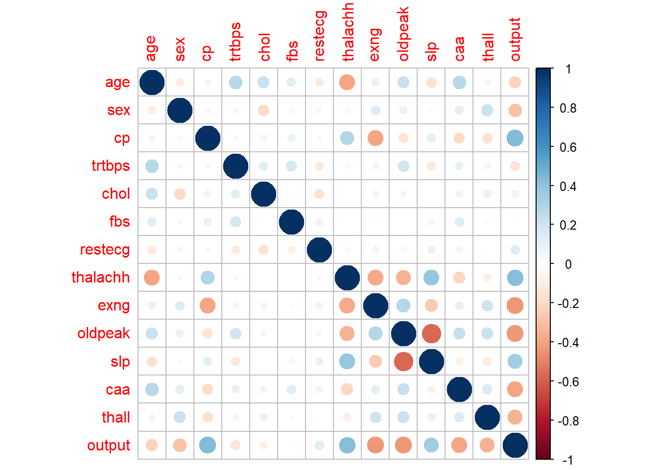
The correlation matrix above shows heart disease to be positively correlated with chest pain, the maximum heart rate achieved, and the incline type of exercise during the testing segment; and negatively correlated with exercise induced angina, and ST depression induced by exercise. I expect any predictive model to take these correlations into account as multi-collinearity violates the assumptions of a normal OLS regression.
The variance-covariance matrix above may suggest that scaling features between 0 and 1 may be useful but I’m unsure if this is applicable and/or it makes it more difficult to interpret any model or coefficients afterwards.
Age distribution
heart %>%
  ggplot(aes(age)) +
  geom_histogram(alpha = 0.5, fill = "dodgerblue",binwidth = 5)+
  geom_vline(xintercept = mean(heart$age),lty = 2)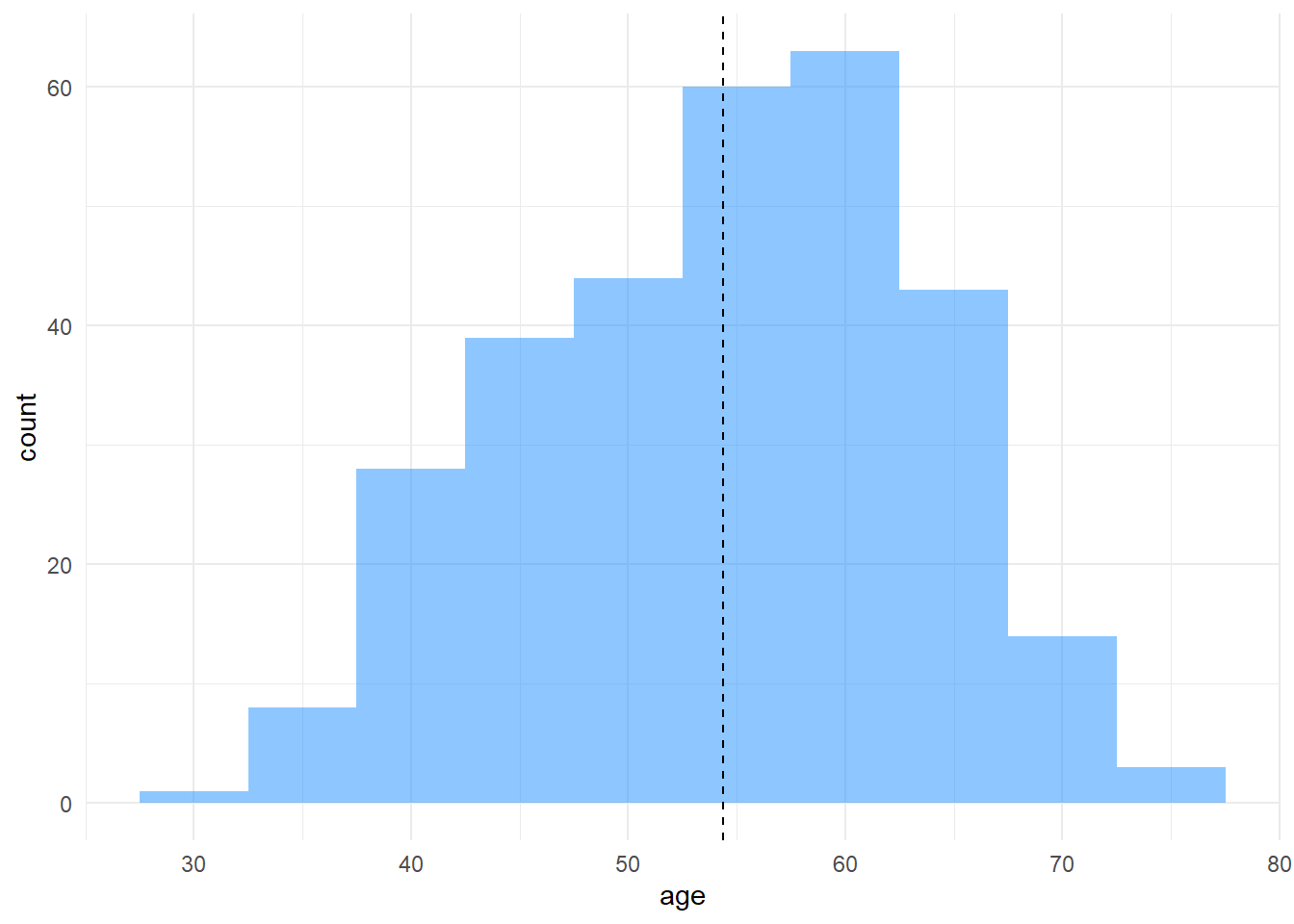
heart %>%
  ggplot(aes(age))+
  geom_density()+
  geom_vline(xintercept = mean(heart$age),lty = 2)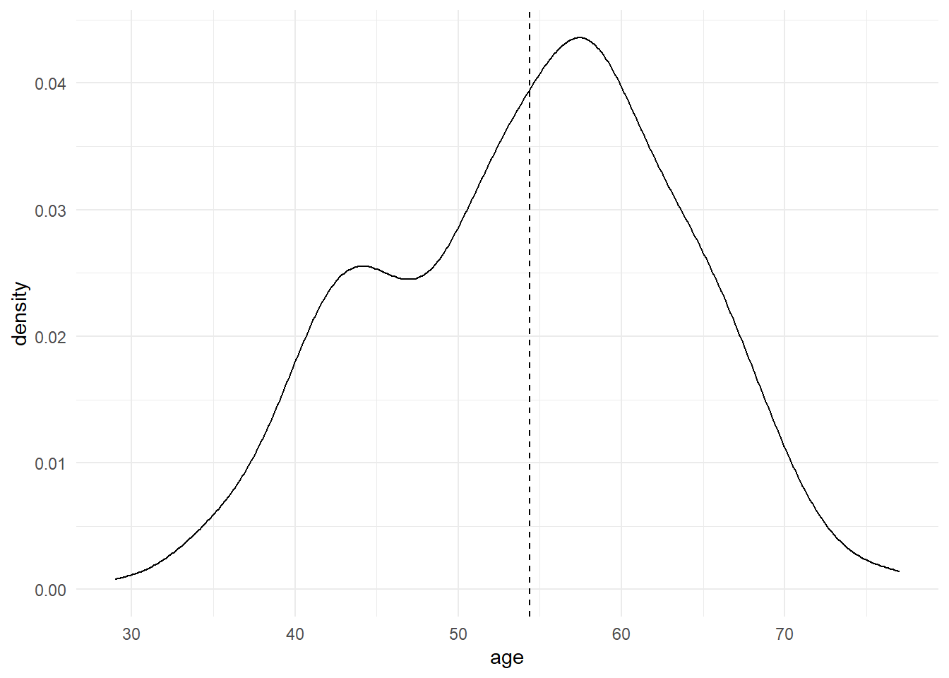
The observations within the dataset tends to skew older ages.
Sex distribution
heart %>%
  count(sex)
## # A tibble: 2 x 2
## sex n
## <dbl> <int>
## 1 0 96
## 2 1 207There are around twice the amount of men featured in the dataset compared to women.
Chest pain distribution
heart %>%
  ggplot(aes(cp))+
  geom_histogram(fill = "dodgerblue")+
  ggtitle("Chest pain", subtitle = "chest pain type (1 = typical angina; 2 = atypical angina; 3 = non-anginal pain; 0 = asymptomatic)")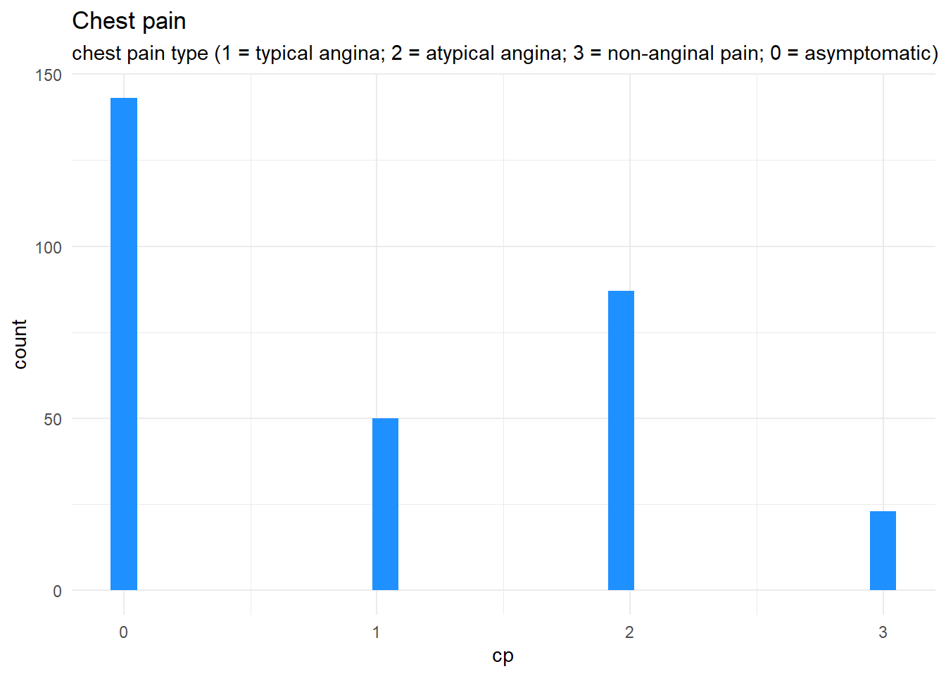
Resting blood pressure
heart %>%
ggplot(aes(trtbps))+
geom_histogram(fill = "dodgerblue")+
ggtitle("Resting blood pressure", subtitle = "resting blood pressure (in mm Hg on admission to the hospital)")+
geom_errorbarh(aes(xmin = 90, xmax = 120, y = 20),height = 4)+
annotate("text",label = "NHS 'normal' range", x = 105, y = 22)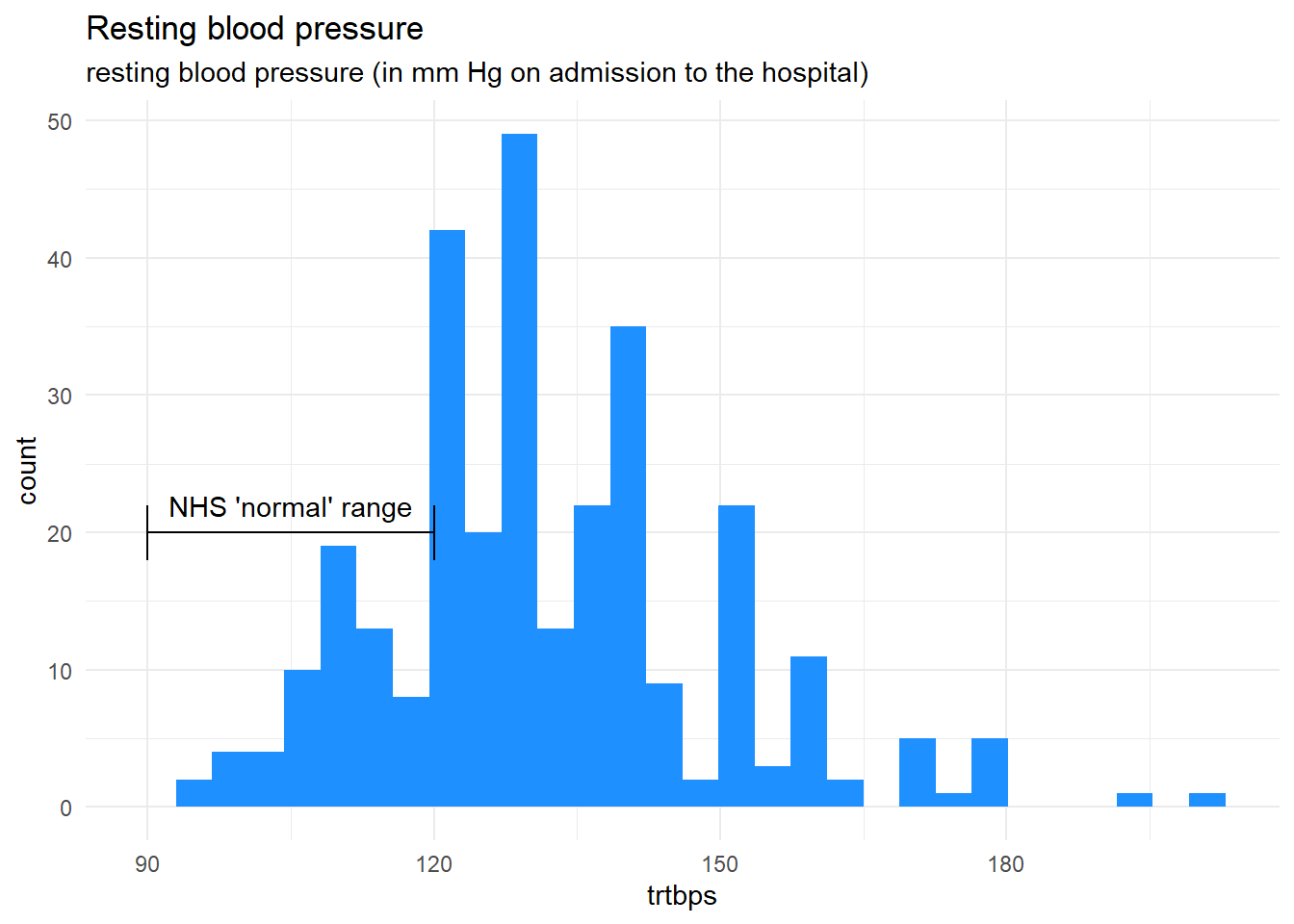 There are a few observations with very high outlier resting blood pressure. According to the NHS, a normal range for resting blood pressure in between 90 and 120.
heart %>%
  filter(trtbps>120) %>%
  count()
## # A tibble: 1 x 1
## n
## <int>
## 1 206The dataset skews heavily 67.99% outside of the ‘normal’ range for resting blood pressure.
Cholestoral levels
heart %>%
ggplot(aes(chol)) +
geom_histogram(fill = "dodgerblue") +
ggtitle("Cholestoral levels",subtitle = "serum cholestoral in mg/dl")+
geom_errorbarh(aes(xmin = 125, xmax = 200, y = 20),height = 2) +
annotate("text",label = "healthy", x = 162.5, y = 22)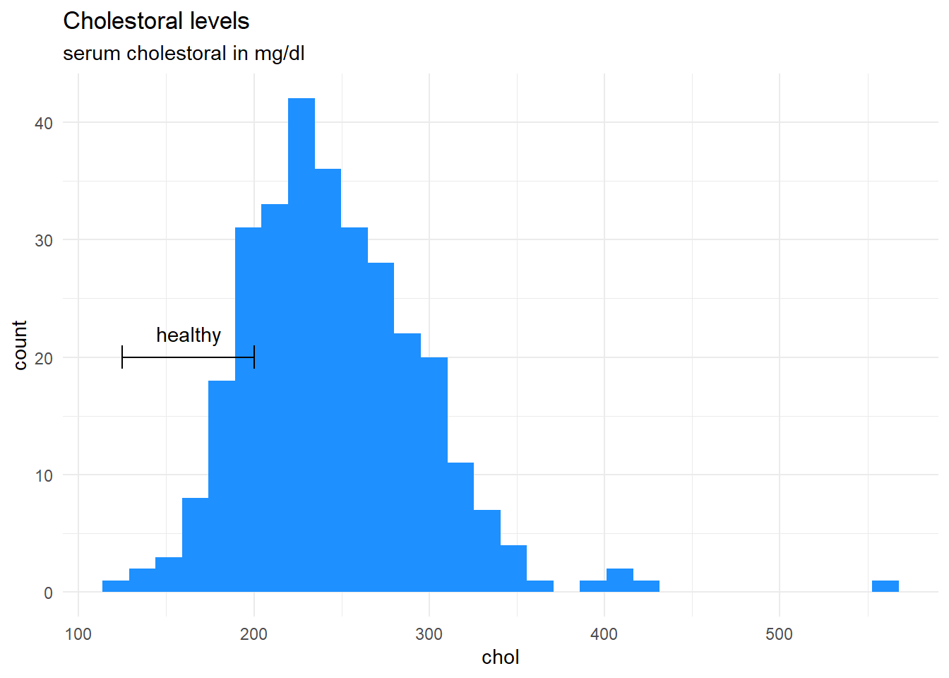 The normal range for cholesterol levels according to medicinenet.com is 125 to 200 mg/dL for men and women over age 20. Most of the observations fall outside of this range. There are very high outliers within the dataset with levels above 400 mg/dL.
heart %>%
ggplot(aes(chol, fill = paste(output))) +
geom_histogram() +
ggtitle("Cholestoral levels",subtitle = "serum cholestoral in mg/dl, faceted by evidence of heart disease")+
geom_errorbarh(aes(xmin = 125, xmax = 200, y = 5),height = 2) +
annotate("text",label = "healthy", x = 162.5, y = 7)+
facet_grid(~output)+
scale_fill_manual(values = c("dodgerblue","red"),aesthetics = c("fill"))+
theme(legend.position = 'none')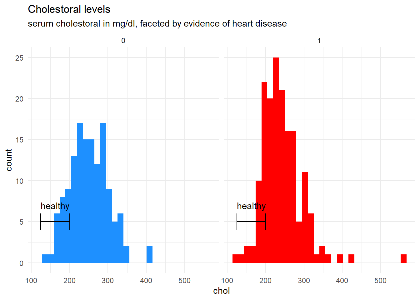 ###
Fitting a model with predictive power
Splitting the dataset into training and testing sets
This allows the model to be applied to previously unseen data to really test for accuracy.
i <- sample(c(rep(0, 0.7 * (nrow(heart)+1)),
              rep(1, 0.3 * (nrow(heart)+1))))


heart_train <- heart[i == 0, ]
heart_test <- heart[i == 1, ]


y <- heart_train$output
#colnames(heart)[1:ncol(heart)-1]
x <- data.matrix(heart_train[, c(colnames(heart)[1:ncol(heart)-1])])
Fitting the Lasso Regression
The reason for choosing this type of model is because non-multicollinearity (predictor variables correlate with each other) is an assumption of an Ordinary Least Squares (OLS) regression. The lasso regression attempts to tackle this problem. The lasso regression includes a shrinkage penalty (\(\lambda\)) to drop certain weakly significant variables from the model and aims to minimise over-fitting.
\[\sum\limits_{i = 1}^{N}(y_i - \hat{y} _i)^2 = \sum\limits_{i = 1}^{N}\left (y_i - \sum\limits_{j = 0}^{p}(\hat{\beta}_j \times x_{i, j})\right)^2 + \lambda \sum\limits_{j = 0}^{p}\mid{\hat{\beta}_j}\mid{}\] The MSE (mean-squared error) formula for the lasso regression above takes the form of a cost or optimisation function. The larger the coefficients, the greater the MSE is, and the greater the model is penalised. The model requires an optimisation of lambda \(\lambda\) to shrink the absolute value of the coefficients \(\hat{\beta}_j\) and optimise for the MSE. This penalty or shrinkage of the coefficients helps to reduce the models complexity and helps to reduce the impact of multi-collinearity between variables.
library(glmnet)
heart_model <- cv.glmnet(x, y, alpha = 1)

best_lambda <- heart_model$lambda.min
Minimising MSE for an appropriate \(\lambda\) and coefficient matrix
plot(heart_model)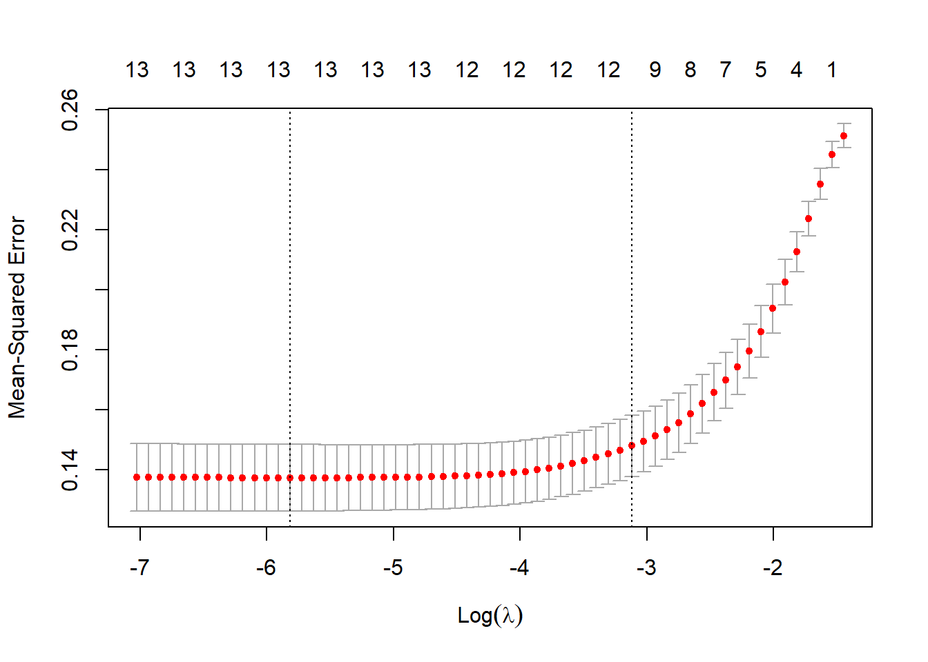
best_model <- glmnet(x, y, alpha = 1, lambda = best_lambda)
coef(best_model)
## 14 x 1 sparse Matrix of class "dgCMatrix"
## s0
## (Intercept) 1.004286311
## age -0.001653948
## sex -0.183465731
## cp 0.137192809
## trtbps -0.003158950
## chol -0.000115763
## fbs 0.138430133
## restecg 0.055071514
## thalachh 0.002966605
## exng -0.110693451
## oldpeak -0.063141927
## slp 0.065677074
## caa -0.053495136
## thall -0.161988579There may be coefficients above that have been reduced to zero because of the nature of the Lasso regression model used. The Lasso regression is often implemented when there are lots of features and over-fitting a model may become a problem in producing an accurate model. Coefficients tending to zero are dropped from the model completely. There may be greater or fewer coefficients dropped depending on the sampling of the training dataset.
Measuring the R-Squared value of the lasso regression model
heart_test_x <- data.matrix(heart_test[, c(colnames(heart)[1:ncol(heart)-1])])

heart_test_y <- heart_test$output

predictions <- predict(best_model, s = best_lambda, newx = heart_test_x)

sst <- sum((y - mean(y))^2) # sum of squares total

sse <- sum((predictions - heart_test_y)^2) # sum of squares error

rsq <- 1 - sse/sst # r-squared

rsq
## [1] 0.7583019The R-squared turns out to be 0.7583. That is, the best model was able to explain 75.83% of the variation in the response values of the training data.
Confusion matrix (how correct was our model?)
full_results <- cbind(data.frame(heart_test_y),predictions, heart_test_x) %>%
  rename("prediction" = "1",
         "output" = "heart_test_y")

confusion_matrix <- full_results %>%
  mutate(correct_prediction = ifelse(output == round(prediction,0),"CORRECT","INCORRECT"),
         prediction_adj = round(prediction,0))
# These packages include useful ML tidying functions
library(caret)
library(InformationValue)optimal <- optimalCutoff(actuals = confusion_matrix$output, predictedScores = confusion_matrix$prediction)
# The InformationValue::optimalCutoff function attempts to predict a better rounding of probability. This may be more accurate than simply rounding to the nearest integer.
optimal## [1] 0.454176(cf <- confusion_matrix %>%
count(correct_prediction))## correct_prediction n
## 1 CORRECT 76
## 2 INCORRECT 15The lasso regression is correct for 83.52% of the testing observations.
Confusion matrix metrics
confusionMatrix(confusion_matrix$output, confusion_matrix$prediction)## 0 1
## 0 31 4
## 1 11 45sensitivity(confusion_matrix$output, confusion_matrix$prediction)## [1] 0.9183673specificity(confusion_matrix$output, confusion_matrix$prediction)## [1] 0.7380952misClassError(confusion_matrix$output, confusion_matrix$prediction)## [1] 0.1648The model has a misclassification rate of 16.48% which is quite reasonable for predicting if someone is at greater risk of heart disease.