Load the weekly Data
Download the weekly data and make available in the tt object.
library(lubridate)## Warning: package 'lubridate' was built under R version 4.0.4##
## Attaching package: 'lubridate'## The following objects are masked from 'package:base':
##
## date, intersect, setdiff, uniontt <- tt_load("2021-04-20")## --- Compiling #TidyTuesday Information for 2021-04-20 ----## --- There is 1 file available ---## --- Starting Download ---##
## Downloading file 1 of 1: `netflix_titles.csv`## --- Download complete ---netflix_titles <- tt$netflix_titles %>%
separate(duration, c("duration", "duration_units"), sep = " ", convert = TRUE) %>%
mutate(date_added = mdy(date_added),
year_added = year(date_added)) %>%
mutate(mature = rating %in% c("TV-MA", "R", "NC-17")) netflix_titles %>%
ggplot(aes(release_year, fill = type)) +
geom_histogram(binwidth = 5) +
facet_wrap(~ type, ncol = 1, scales = "free_y")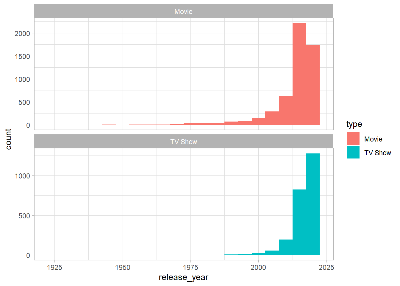
netflix_titles %>%
  #count(year = 2 * (release_year %/% 2), type) %>%
  count(year = release_year, type) %>%
  group_by(type) %>%
  mutate(percent = n / sum(n)) %>%
  ggplot(aes(year, percent, color = type)) +
  geom_line()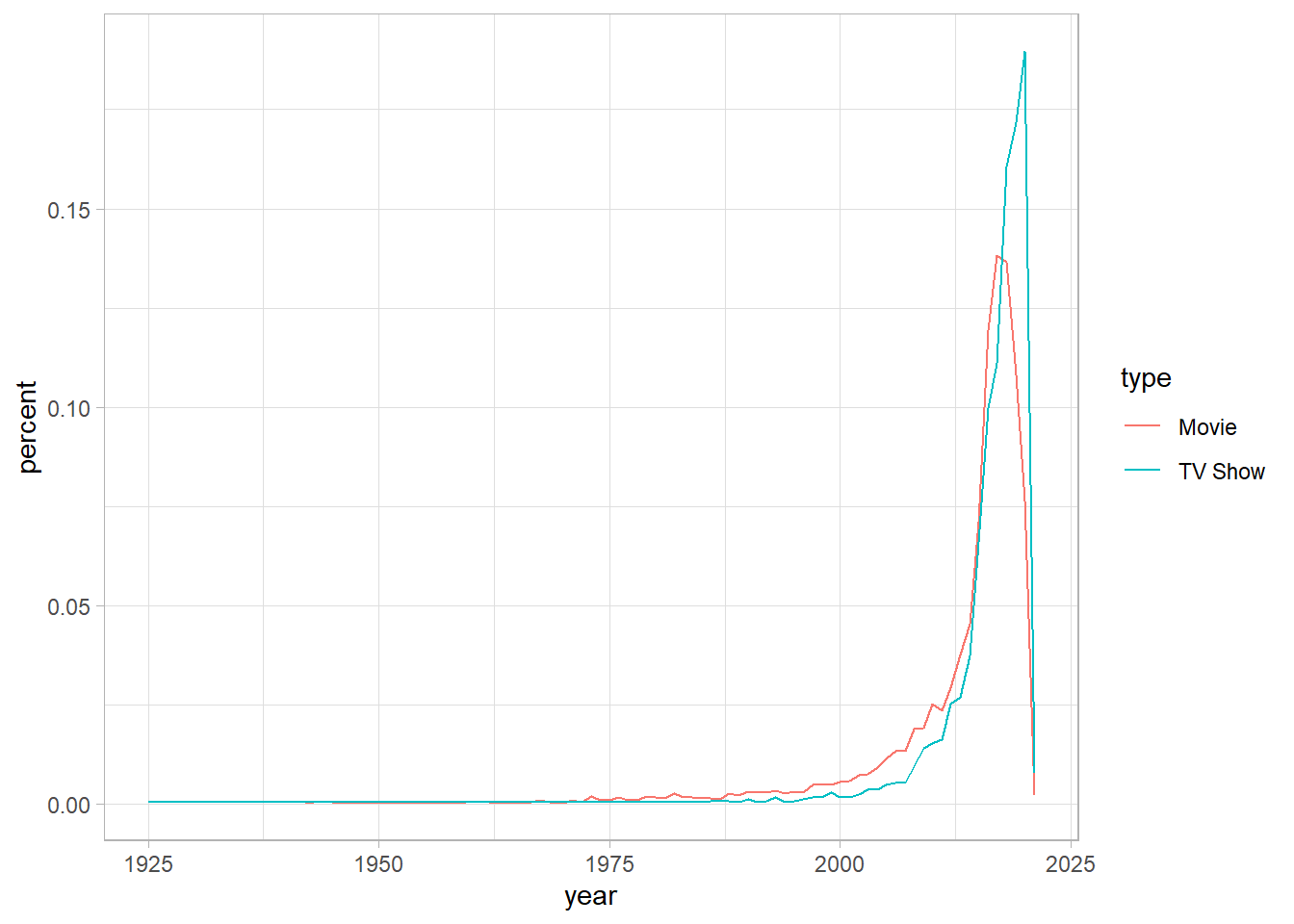
netflix_titles %>%
  filter(type == "Movie") %>%
  mutate(decade = 10 * (release_year %/% 10)) %>%
  ggplot(aes(decade, duration, group = decade)) +
  geom_boxplot()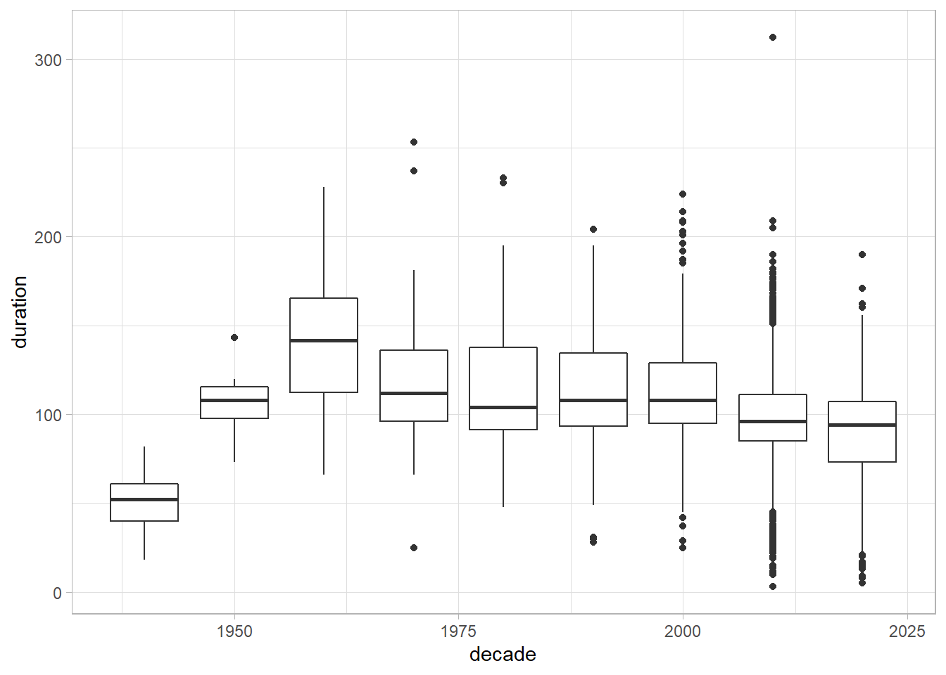
summarize_titles <- function(tbl) {
  tbl %>%
    summarize(n = n(),
              median_duration = median(duration),
              median_year = median(release_year)) %>%
    arrange(desc(n))
}
netflix_titles %>%
count(rating, sort = TRUE)## # A tibble: 15 x 2
## rating n
## <chr> <int>
## 1 TV-MA 2863
## 2 TV-14 1931
## 3 TV-PG 806
## 4 R 665
## 5 PG-13 386
## 6 TV-Y 280
## 7 TV-Y7 271
## 8 PG 247
## 9 TV-G 194
## 10 NR 84
## 11 G 39
## 12 <NA> 7
## 13 TV-Y7-FV 6
## 14 UR 5
## 15 NC-17 3netflix_titles %>%
separate_rows(listed_in, sep = ", ") %>%
group_by(type, genre = listed_in) %>%
summarize_titles() %>%
filter(type == "Movie") %>%
filter(genre != "Movies") %>%
mutate(genre = fct_reorder(genre, median_duration)) %>%
ggplot(aes(median_duration, genre)) +
geom_col()## `summarise()` has grouped output by 'type'. You can override using the `.groups` argument.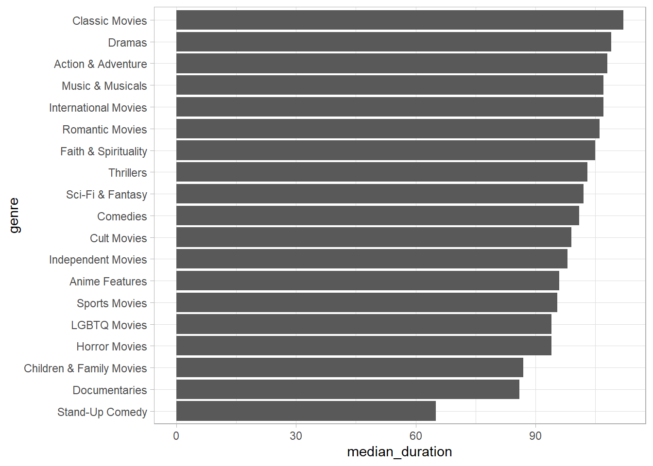
head(netflix_titles$date_added)## [1] "2020-08-14" "2016-12-23" "2018-12-20" "2017-11-16" "2020-01-01"
## [6] "2017-07-01"Date added
netflix_titles %>%
  filter(!is.na(date_added)) %>%
  arrange(date_added) %>%
  select(type, title, date_added)
## # A tibble: 7,777 x 3
## type title date_added
## <chr> <chr> <date>
## 1 Movie To and From New York 2008-01-01
## 2 TV Show Dinner for Five 2008-02-04
## 3 Movie Just Another Love Story 2009-05-05
## 4 Movie Splatter 2009-11-18
## 5 Movie Mad Ron's Prevues from Hell 2010-11-01
## 6 Movie Even the Rain 2011-05-17
## 7 Movie Joseph: King of Dreams 2011-09-27
## 8 Movie A Stoning in Fulham County 2011-10-01
## 9 Movie Adam: His Song Continues 2011-10-01
## 10 Movie Hard Lessons 2011-10-01
## # ... with 7,767 more rowsnetflix_titles %>%
filter(!is.na(date_added)) %>%
count(year_added, type) %>%
ggplot(aes(year_added, n, fill = type)) +
geom_area()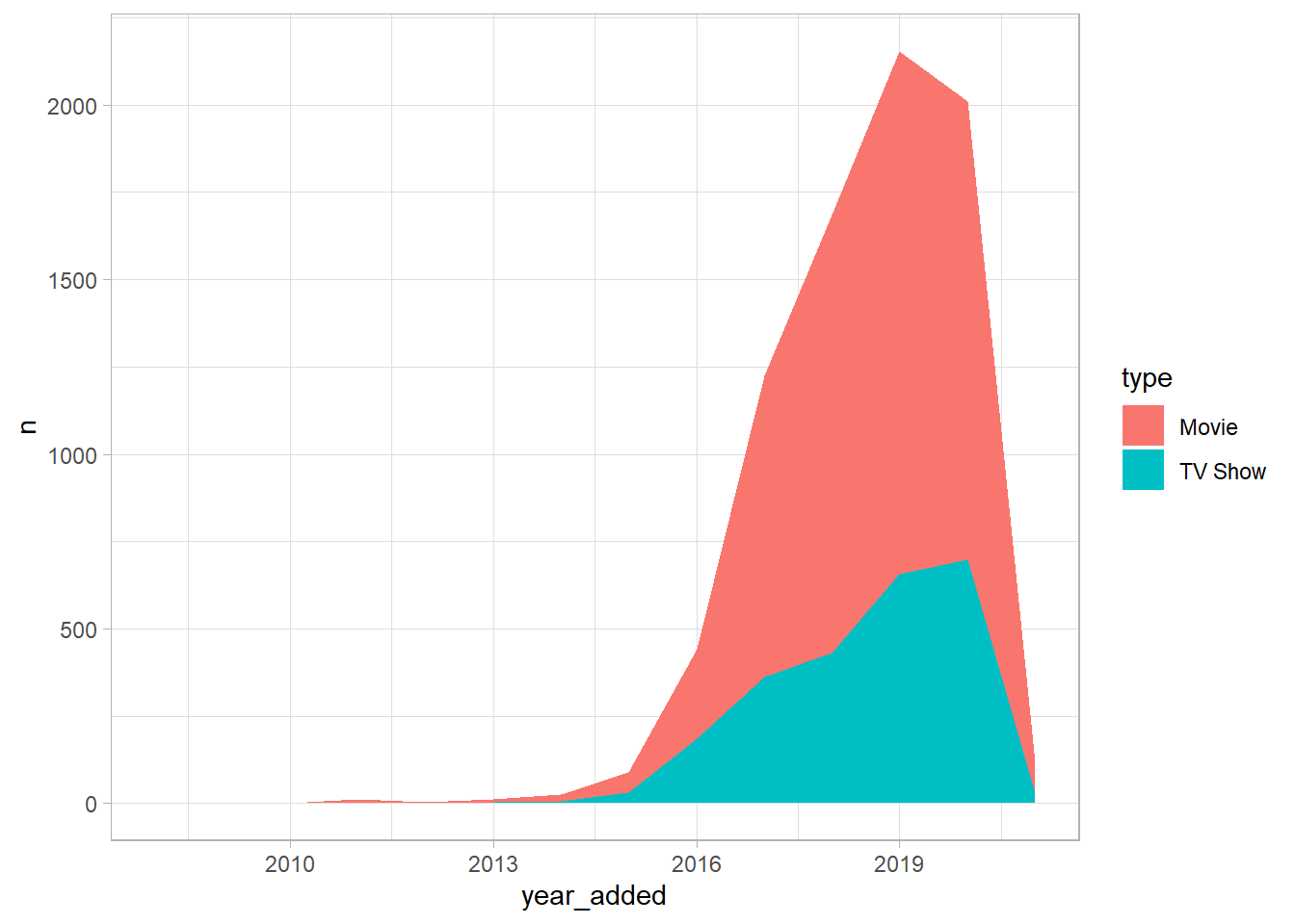
netflix_titles %>%
  filter(year_added >= 2015) %>%
  filter(!is.na(date_added), !is.na(rating)) %>%
  mutate(rating = fct_lump(rating, 5)) %>%
  ungroup() %>%
  count(type, year_added, rating) %>%
  group_by(type, year_added) %>%
  mutate(percent = n / sum(n)) %>%
  ggplot(aes(year_added, percent, fill = rating)) +
  geom_area() +
  facet_wrap(~ type)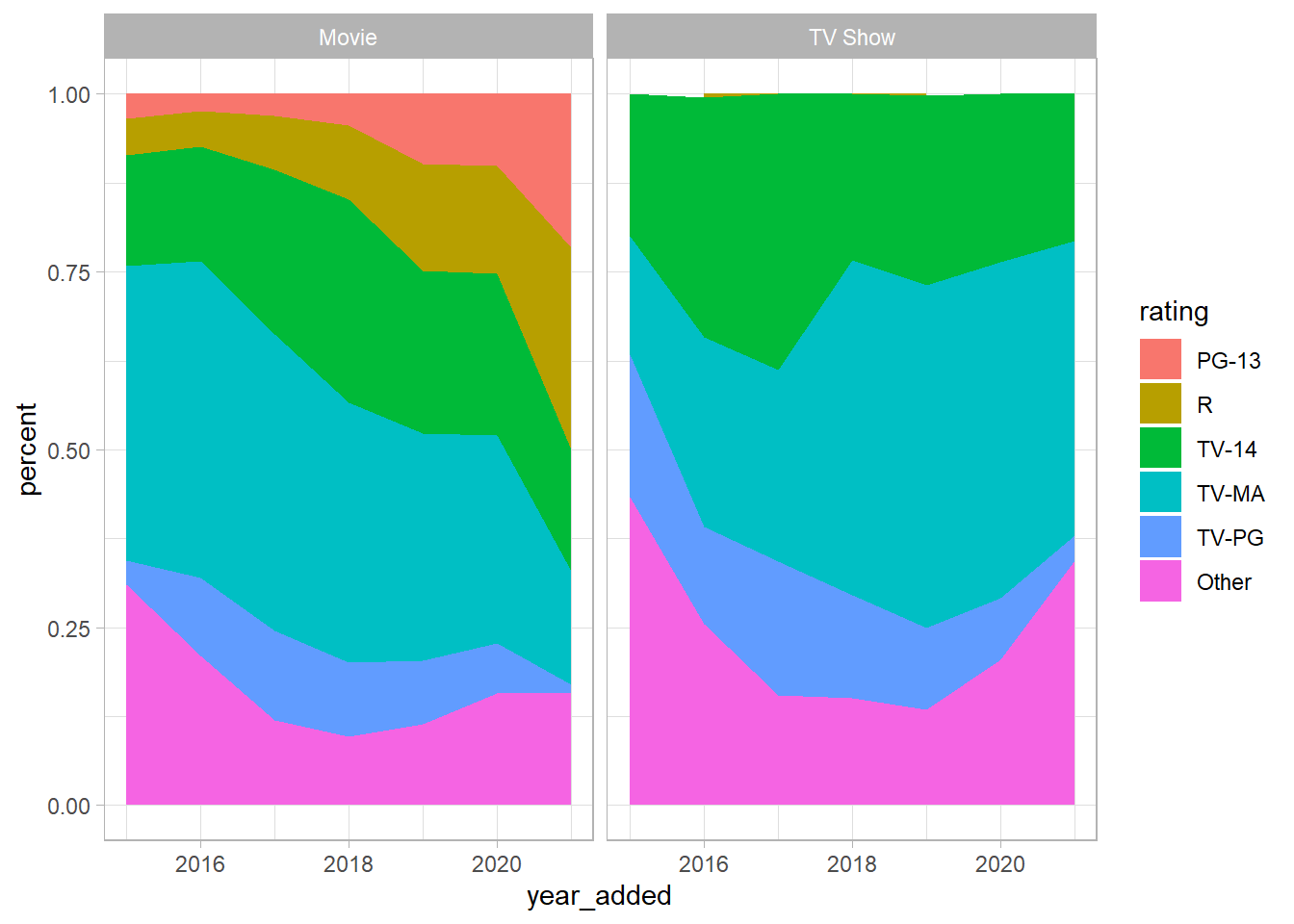
netflix_titles %>%
  filter(!is.na(country)) %>%
  count(country = fct_lump(country, 20),
        type,
        sort = TRUE) %>%
  mutate(country = fct_reorder(country, n)) %>%
  ggplot(aes(n, country, fill = type)) +
  geom_col()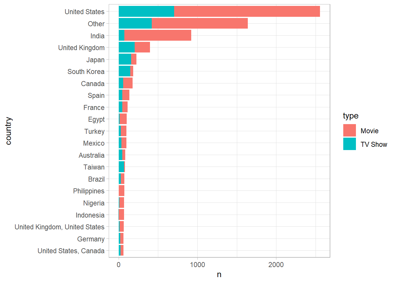
netflix_titles %>%
  filter(!is.na(country)) %>%
  filter(type == "Movie") %>%
  group_by(country) %>%
  summarize_titles()
## # A tibble: 590 x 4
## country n median_duration median_year
## <chr> <int> <dbl> <dbl>
## 1 United States 1850 91 2016
## 2 India 852 127 2014.
## 3 United Kingdom 193 90 2016
## 4 Canada 118 89 2017
## 5 Egypt 89 101 2012
## 6 Spain 89 99 2018
## 7 Turkey 73 104 2015
## 8 Philippines 70 112. 2016
## 9 France 69 95 2017
## 10 Japan 69 98 2016
## # ... with 580 more rowsnetflix_titles %>%
filter(rating %in% c("R", "TV-MA")) %>%
count(country, sort = TRUE)## # A tibble: 399 x 2
## country n
## <chr> <int>
## 1 United States 1244
## 2 India 230
## 3 United Kingdom 199
## 4 <NA> 161
## 5 Spain 111
## 6 South Korea 83
## 7 Japan 82
## 8 France 77
## 9 Canada 76
## 10 Mexico 73
## # ... with 389 more rowsnetflix_titles %>%
filter(!is.na(rating), !is.na(country)) %>%
group_by(type, country = fct_lump(country, 9)) %>%
summarize(n_mature = sum(rating %in% c("R", "TV-MA", "NC-17")),
n = n(),
.groups = "drop") %>%
mutate(pct_mature = n_mature / n,
conf_low = qbeta(.025, n_mature + .5, n - n_mature + .5),
conf_high = qbeta(.975, n_mature + .5, n - n_mature + .5)) %>%
ggplot(aes(pct_mature, country, color = type)) +
geom_point(aes(size = n)) +
geom_errorbar(aes(xmin = conf_low, xmax = conf_high), width = .1) +
scale_x_continuous(labels = percent) +
expand_limits(x = 0) +
labs(x = "% of titles that are R/TV-MA")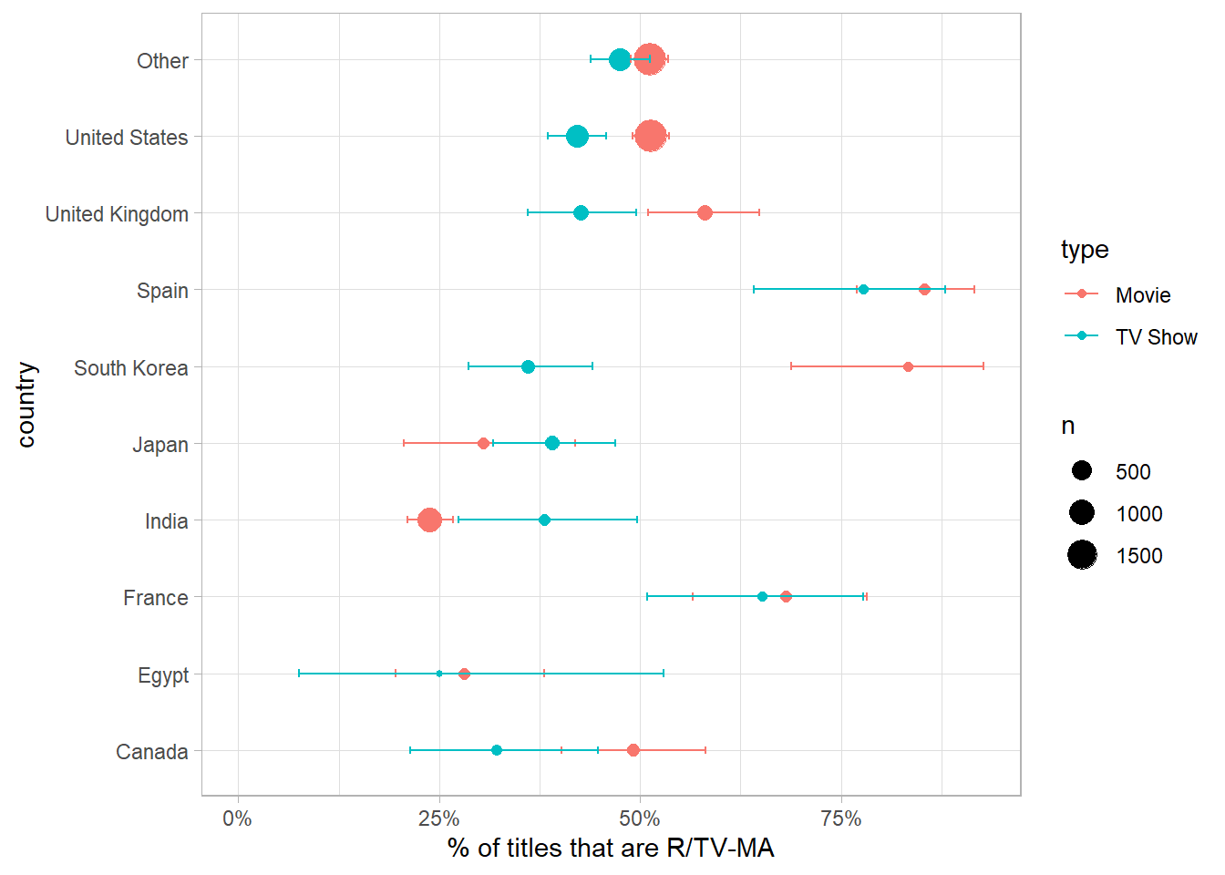
library(tidytext)## Warning: package 'tidytext' was built under R version 4.0.5library(snakecase)## Warning: package 'snakecase' was built under R version 4.0.3library(tidylo)## Warning: package 'tidylo' was built under R version 4.0.5words_unnested <- netflix_titles %>%
unnest_tokens(word, description) %>%
anti_join(stop_words, by = "word")
words_unnested %>%
count(type, word, sort = TRUE) %>%
mutate(type = to_snake_case(type)) %>%
spread(type, n, fill = 0) %>%
mutate(total = movie + tv_show) %>%
arrange(desc(total)) %>%
head(100) %>%
ggplot(aes(movie, tv_show)) +
geom_point() +
geom_text(aes(label = word) , vjust = 1, hjust = 1) +
scale_x_log10() +
scale_y_log10()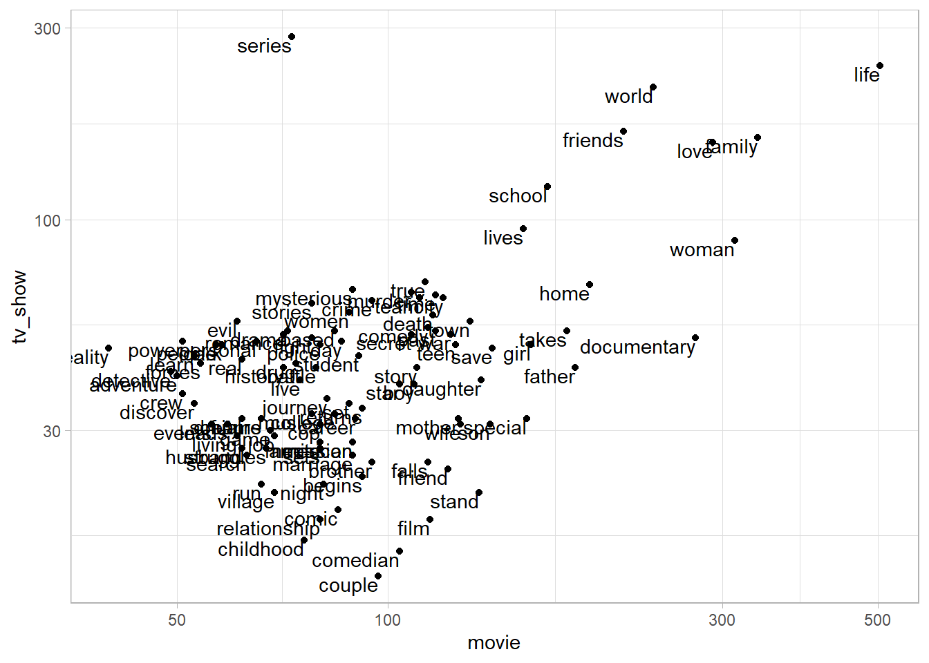
words_unnested %>%
  count(type, word) %>%
  bind_log_odds(type, word, n) %>%
  arrange(desc(log_odds_weighted)) %>%
  group_by(type) %>%
  top_n(10, log_odds_weighted) %>%
  ungroup() %>%
  mutate(word = fct_reorder(word, log_odds_weighted)) %>%
  ggplot(aes(log_odds_weighted, word)) +
  geom_col() +
  facet_wrap(~ type, scales = "free_y")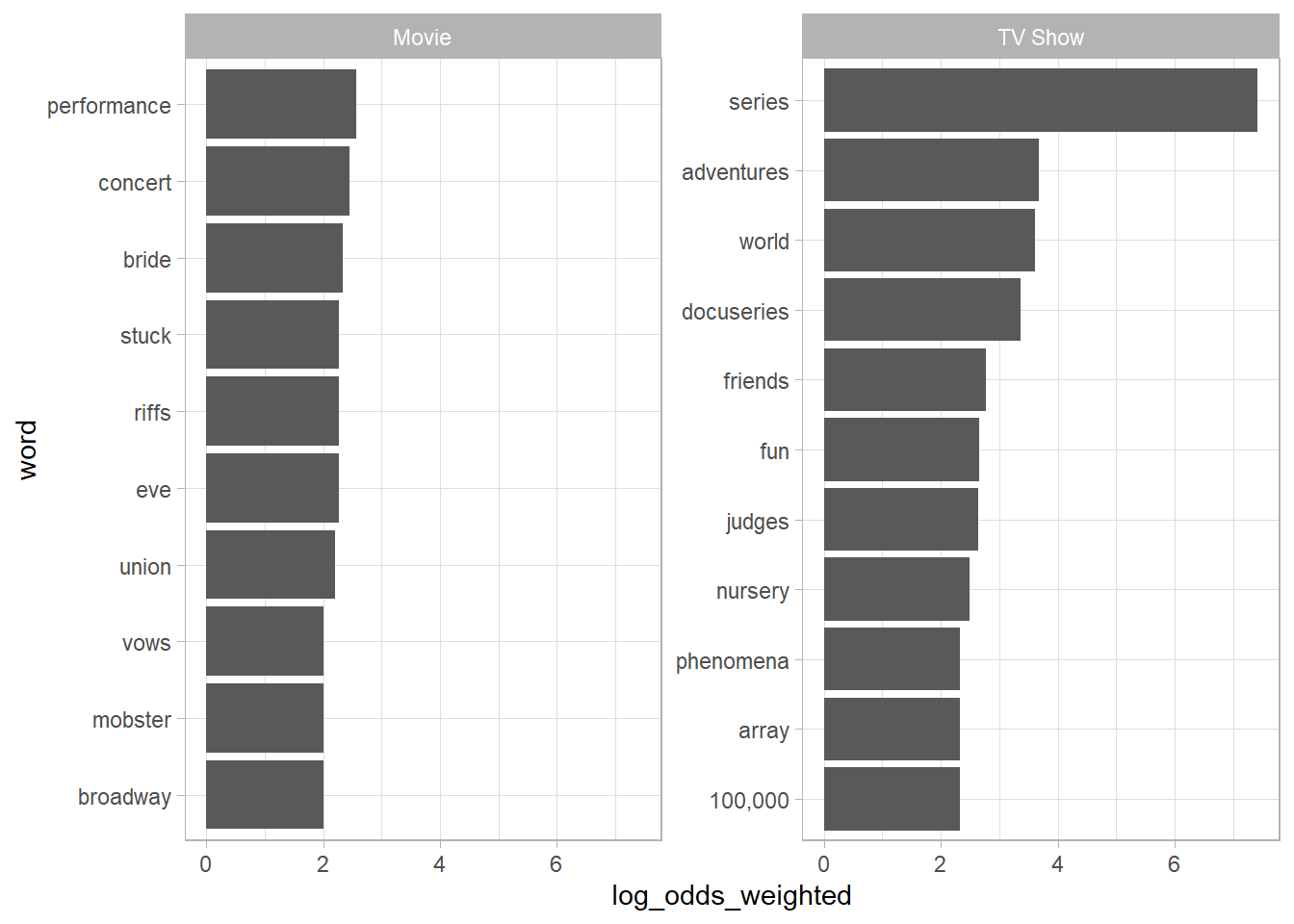
library(widyr)
library(tidygraph)
## Warning: package 'tidygraph' was built under R version 4.0.5##
## Attaching package: 'tidygraph'## The following object is masked from 'package:stats':
##
## filterlibrary(ggraph)## Warning: package 'ggraph' was built under R version 4.0.5set.seed(2021)
words_unnested %>%
distinct(type, title, word) %>%
add_count(word, name = "word_total") %>%
filter(word_total >= 40) %>%
pairwise_cor(word, title, sort = TRUE) %>%
filter(correlation >= .1) %>%
igraph::graph_from_data_frame() %>%
ggraph(layout = "fr") +
geom_edge_link(aes(alpha = correlation)) +
geom_node_point() +
geom_node_text(aes(label = name),
repel = TRUE) +
theme(legend.position = "none")## Warning: `tbl_df()` was deprecated in dplyr 1.0.0.
## Please use `tibble::as_tibble()` instead.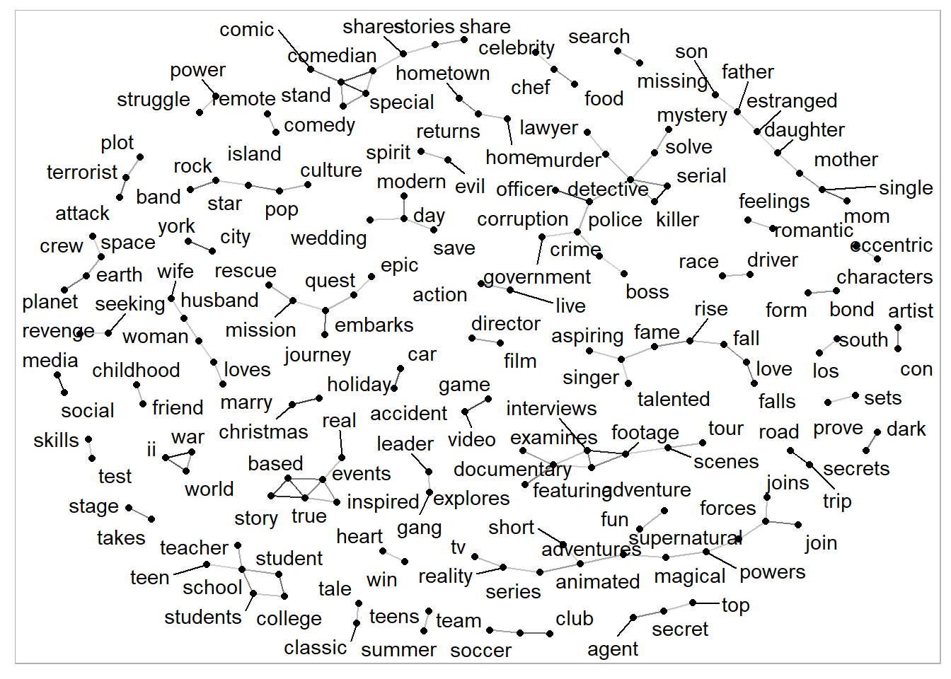
word_genre_log_odds <- words_unnested %>%
  distinct(type, title, word, genre = listed_in) %>%
  add_count(word, name = "word_total") %>%
  filter(word_total >= 25) %>%
  separate_rows(genre, sep = ", ") %>%
  filter(fct_lump(genre, 9) != "Other") %>%
  count(genre, word) %>%
  bind_log_odds(genre, word, n)
word_genre_log_odds %>%
group_by(genre) %>%
top_n(10, log_odds_weighted) %>%
ungroup() %>%
mutate(word = reorder_within(word, log_odds_weighted, genre)) %>%
ggplot(aes(log_odds_weighted, word, fill = genre)) +
geom_col() +
facet_wrap(~ genre, scales = "free_y") +
scale_y_reordered() +
theme(legend.position = "none") +
labs(x = "Log-odds of word's specificity to genre",
y = "")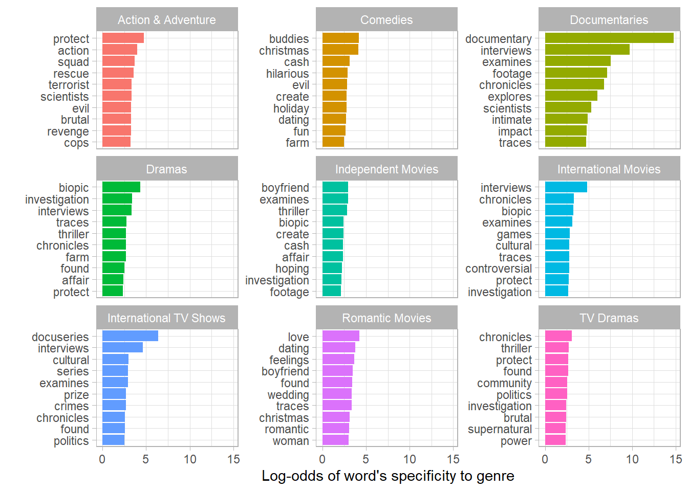
Lasso regression
word_ratings <- words_unnested %>%
  count(type, title, rating, word) %>%
  filter(!is.na(rating)) %>%
  add_count(word, name = "word_total") %>%
filter(word_total >= 30)library(glmnet)## Warning: package 'glmnet' was built under R version 4.0.4## Loading required package: Matrix##
## Attaching package: 'Matrix'## The following objects are masked from 'package:tidyr':
##
## expand, pack, unpack## Loaded glmnet 4.1-1library(broom)## Warning: package 'broom' was built under R version 4.0.5other_features <- netflix_titles %>%
select(title, director, cast, genre = listed_in, country) %>%
gather(feature_type, feature, director, cast, genre, country) %>%
filter(!is.na(feature)) %>%
separate_rows(feature, sep = ", ") %>%
mutate(feature_type = str_to_title(feature_type)) %>%
unite(feature, feature_type, feature, sep = ": ") %>%
add_count(feature, name = "feature_count") %>%
filter(feature_count >= 10)
feature_matrix <- word_ratings %>%
mutate(feature = paste("Description:", word)) %>%
bind_rows(other_features) %>%
cast_sparse(title, feature)
y <- netflix_titles$mature[match(rownames(feature_matrix), netflix_titles$title)]
mod <- cv.glmnet(feature_matrix, y, family = "binomial")
plot(mod)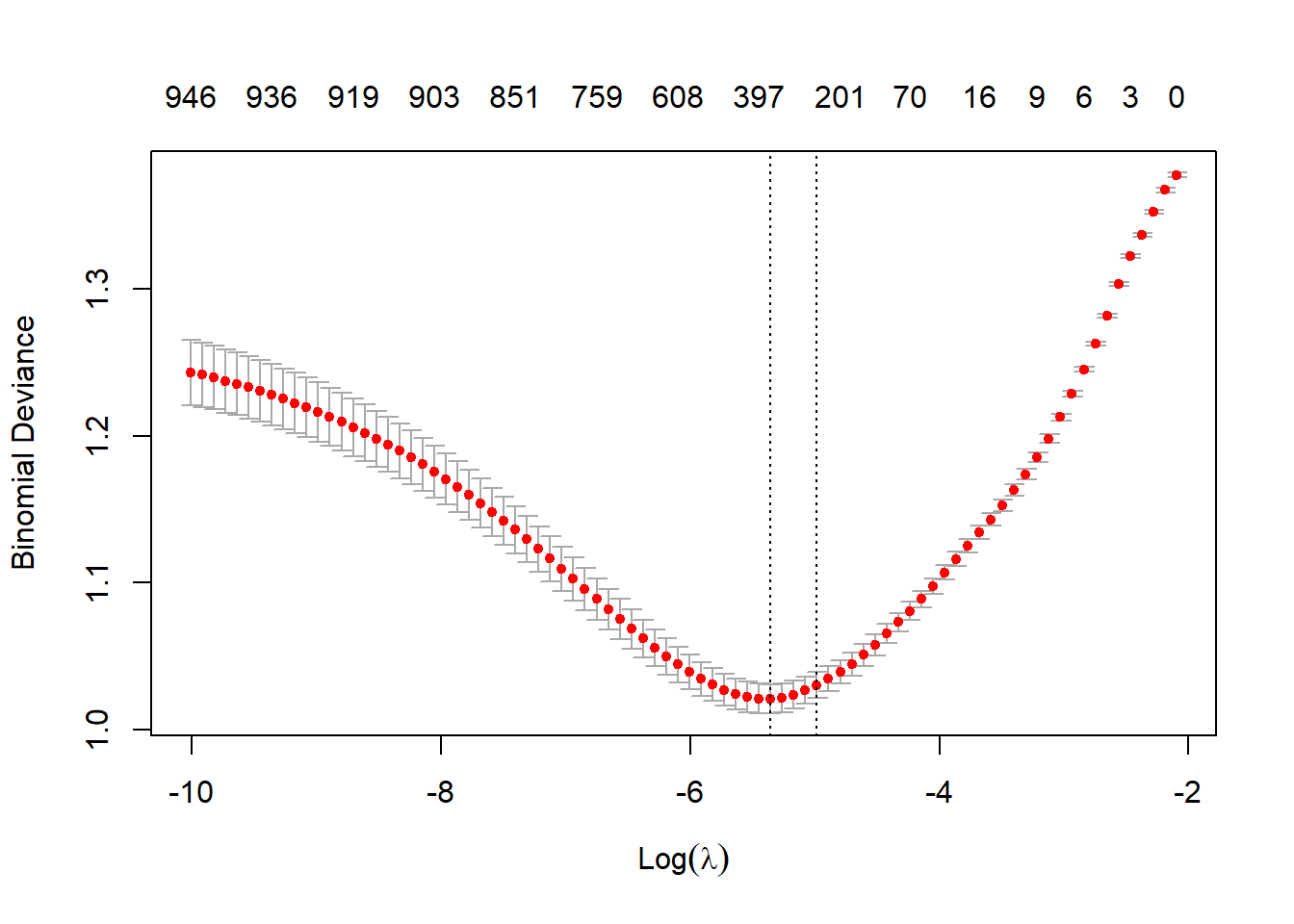
mod$glmnet.fit %>%
  tidy() %>%
  separate(term, c("feature_type", "feature"), sep = ": ") %>%
  filter(lambda == mod$lambda.1se) %>%
  top_n(60, abs(estimate)) %>%
  mutate(feature = fct_reorder(feature, estimate)) %>%
  ggplot(aes(estimate, feature, fill = feature_type)) +
  geom_col() +
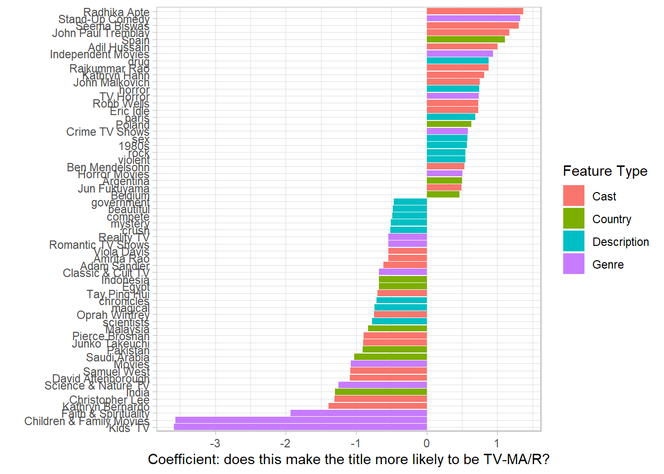
  labs(x = "Coefficient: does this make the title more likely to be TV-MA/R?",
       y = "",
       fill = "Feature Type")
## Warning: Expected 2 pieces. Missing pieces filled with `NA` in 86 rows [1, 2, 3,
## 4, 5, 6, 7, 8, 9, 10, 11, 12, 13, 14, 15, 16, 17, 18, 19, 20, ...].