https://doi.org/10.1016/j.dib.2018.11.111
divide01 <- function(x){
  return(x/100)
}

data <- read.csv("hardness.csv") %>%
  mutate(Al=divide01(Al),
         Co=divide01(Co),
         Cr=divide01(Cr),
         Cu=divide01(Cu),
         Fe=divide01(Fe),
         Ni=divide01(Ni))
data_ordered <- read.csv("hardness.csv") %>%
  mutate(Al=divide01(Al),
         Co=divide01(Co),
         Cr=divide01(Cr),
         Cu=divide01(Cu),
         Fe=divide01(Fe),
         Ni=divide01(Ni)) %>%
  arrange(desc(hardness))

closed <- clo(data, parts = 1:6,total=100)
cx <- acomp(data, c("Al","Co","Cr"))
plot(cx)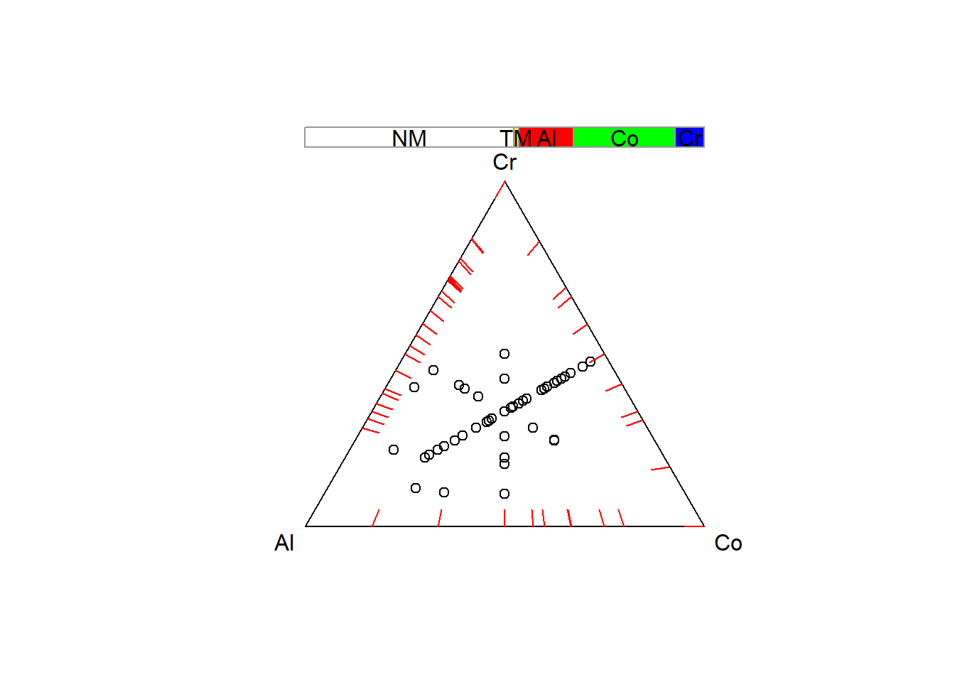
xc <- acomp(data, c("Al","Co","Cr","Cu","Fe","Ni"))
xc_ordered <- acomp(data_ordered, c("Al","Co","Cr","Cu","Fe","Ni"))
plot(xc)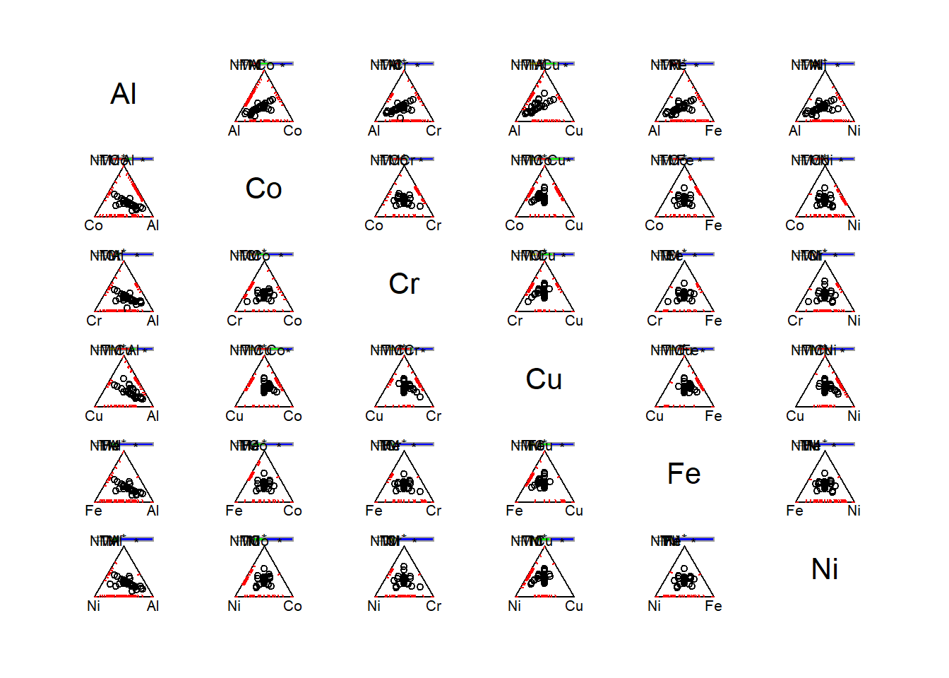
barplot.acomp(xc)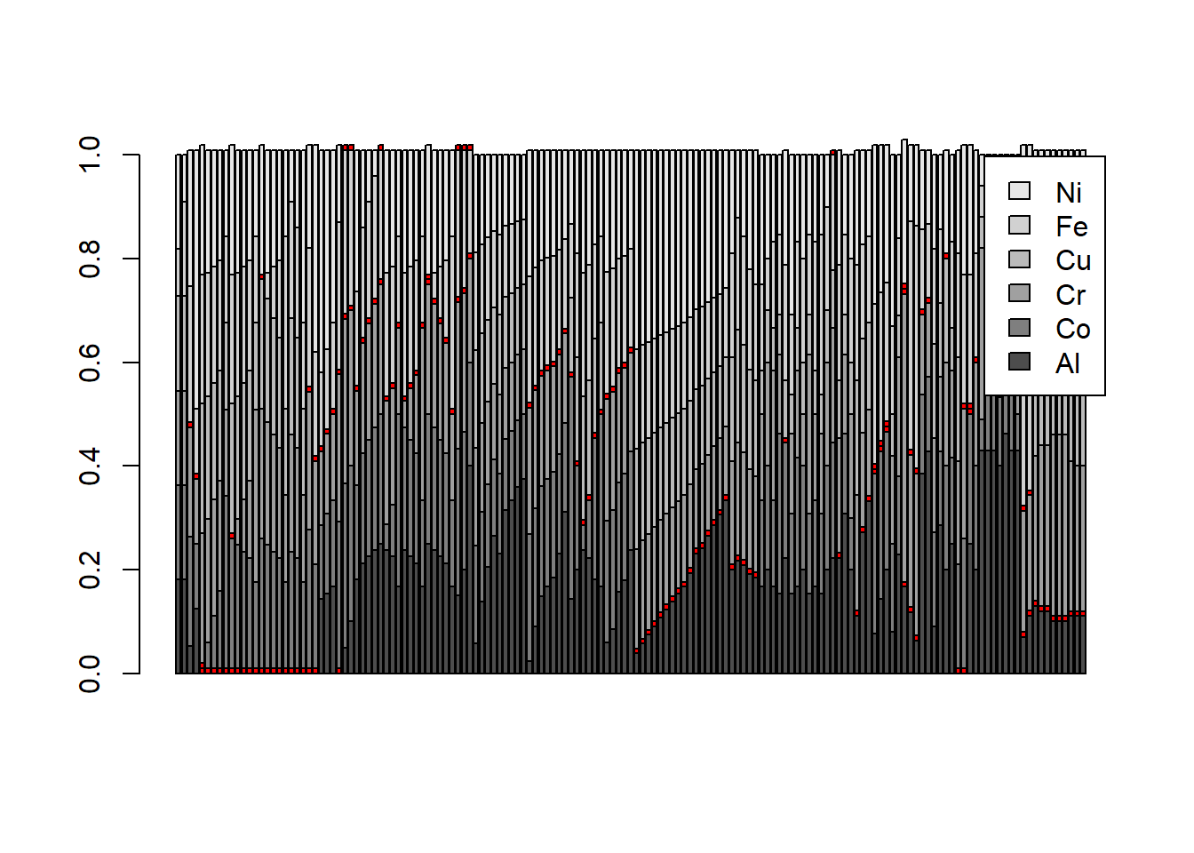
Order of hardness desc
barplot.acomp(xc_ordered)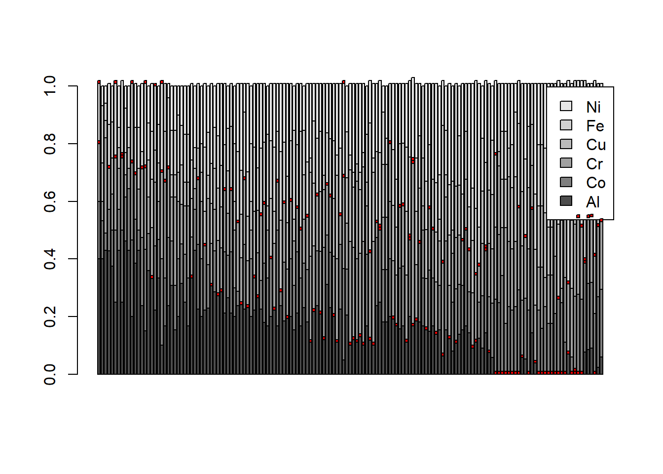
Possibly drop copper and nickel
library(httr)
raw_dd <- read.table(text=content(GET("https://gist.githubusercontent.com/MrFlick/c1183c911bc5398105d4/raw/715868fba2d0d17a61a8081de17c468bbc525ab1/elements.txt")), sep=",", header=TRUE) %>%
  mutate(ElementName=ifelse(ElementName=="Sulfer","Sulfur",ElementName),
         ElementName=ifelse(ElementName=="Phosphorous","Phosphorus",ElementName),
         ElementName=ifelse(ElementName=="Flourine","Fluorine",ElementName))
data <- read_xlsx("melting_points.xlsx", sheet = 'Sheet2')
colnames(raw_dd) <- c(colnames(raw_dd)[1:7],"element",colnames(raw_dd)[9:13])
dd <- raw_dd %>%
left_join(data, by = "element") %>%
mutate(CTE_ppm=CTE*1000000,
CTE_ppm=as.numeric(CTE_ppm),
scaled_cte=CTE_ppm,
scaled_cte=ifelse(scaled_cte>8,8,scaled_cte),
scaled_cte=ifelse(scaled_cte<4.5,4.4,scaled_cte),
new_structure=ifelse(crystal_structure %in% c("Body-centered Cubic","Face-centered Cubic","Simple Hexagonal"),crystal_structure,NA))dd %>%
ggplot(aes(Column,-Row)) +
geom_tile(aes(fill=crystal_structure), color="black") +
geom_text(aes(Column, -Row,label= symbol))+
theme_void()+
labs(
fill = "Crystal Structure"
) +
annotate("text", x = 7, y = 0.2, label = "Periodic Table of the elements", size = 5)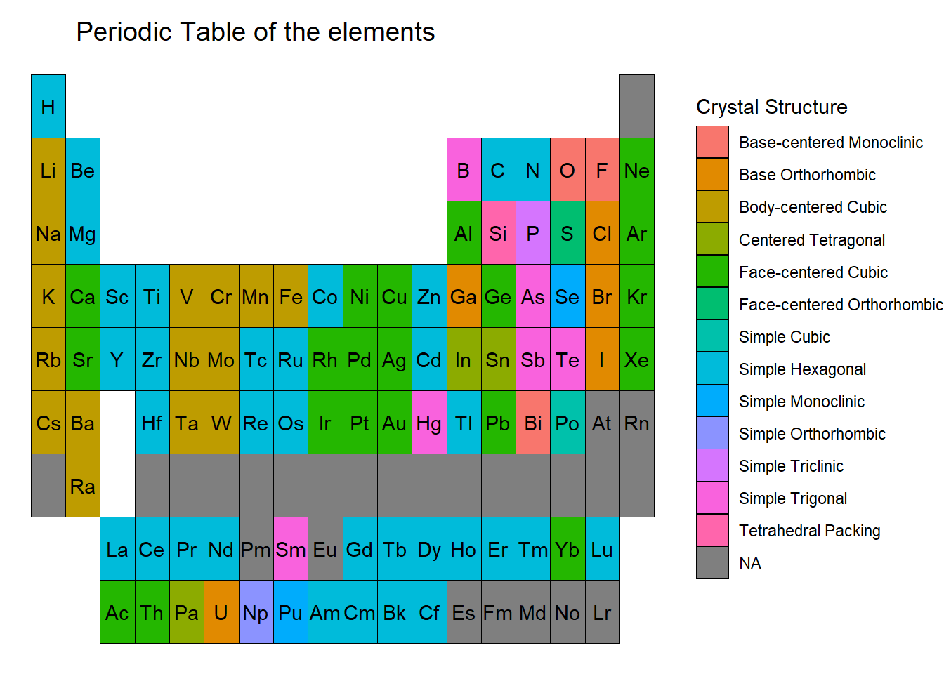
(p<-dd %>%
  filter(!is.na(symbol)) %>%
  #filter(!crystal_structure %in% c("Base-centered Monoclinic","Centered Tetragonal")) %>%
  ggplot(aes(Column, -Row))+
  geom_tile(aes(fill=scaled_cte), color="black",size=1) +
  geom_rect(aes(xmin=Column-0.3,xmax=Column+0.3,ymin=-Row-0.2,ymax=-Row+0.3,colour=new_structure),size=1,lty=1,fill="black")+
    #geom_text(aes(label="",colour=new_structure), na.rm = T,size=12,nudge_y = 0.3)+
  geom_text(aes(label=symbol),colour="yellow",nudge_y = +0.05)+
  geom_text(aes(label=CTE_ppm),colour="black",nudge_y = -0.35)+
  scale_fill_gradient(low = "red",high = "green")+
  labs(fill = expression(paste("CTE", 10^6)),
    colour="") +
  annotate("text", x = 7, y = 0.2, label = "Periodic Table of the elements", size = 5))+
  theme_void()+
  theme(legend.position="bottom")+
  scale_colour_discrete(na.translate = F)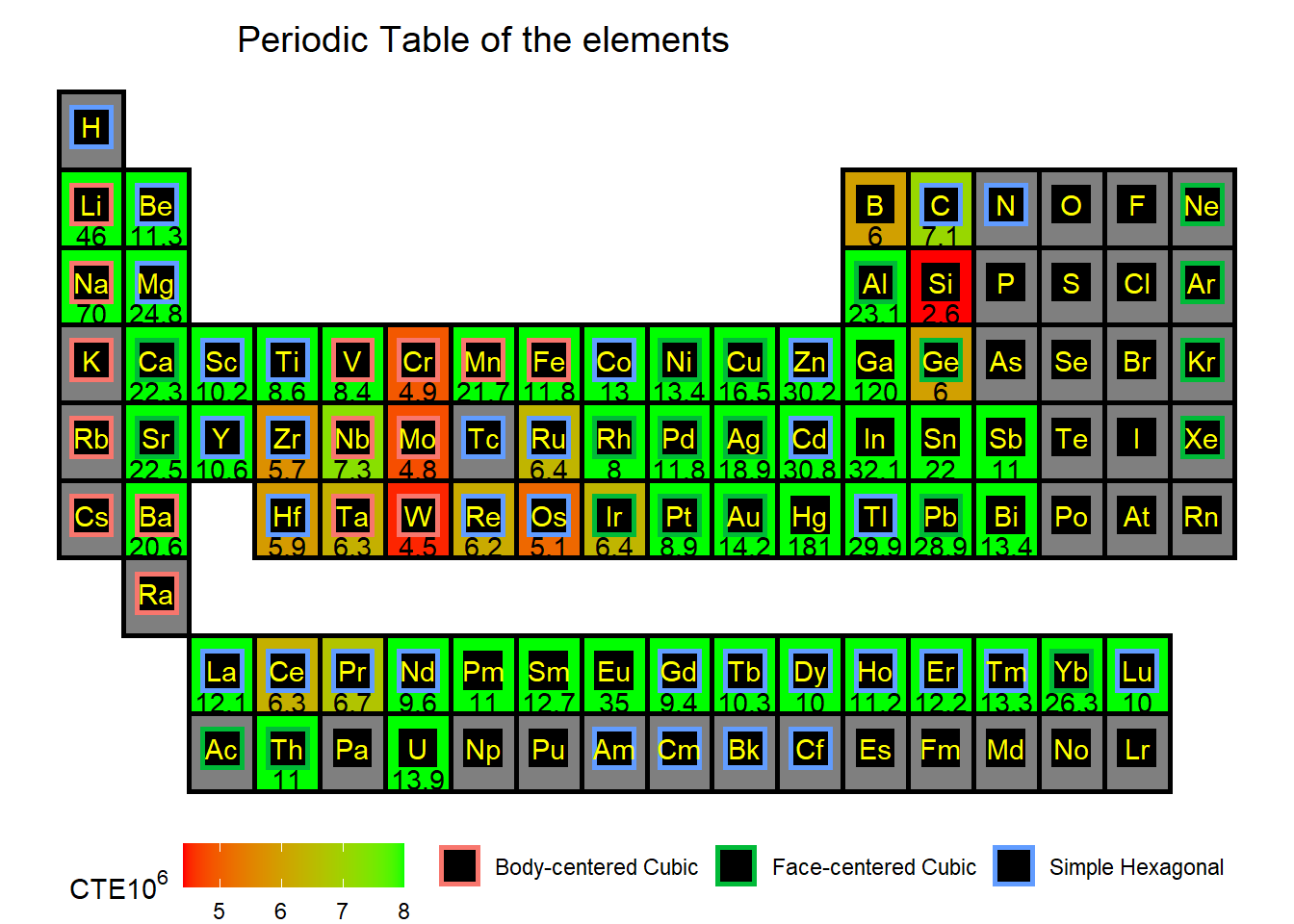
f1 <- function(x){
  return(1/(16.6*3*(x+273)))
}

library(plotly)
library(ggrepel)
data %>%
  ggplot(aes(mp, CTE, label=element))+
  geom_point()+
  stat_function(fun=f1)+
  lims(
    x=c(1500,4000),
    y=c(0,0.000025)
  )+
  theme(legend.position = "none")+
  ggrepel::geom_text_repel()+
  theme_bw()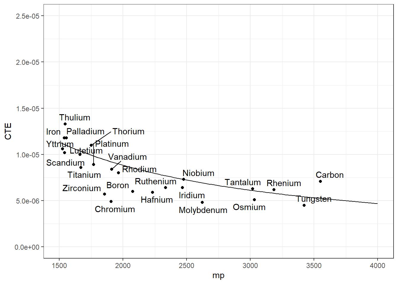
Predictive modelling
Compositional data can be transformed to satisfy linearity by using logratio transformations for representation in a Euclidean space. Additive, isometric, and centre logratio transformations are available.
The transformations give the same coefficients for the multi-variate regressions so we will stick with the additive logratio defined as: \[alr(x) = \left [\log\frac{x_1}{x_n},\ldots,\log\frac{x_{n-1}}{x_n}\right]\]
These transformation functions are available within the ‘compositions’ R package. Ratio transformations have issues with zero-value elements.
PRINCIPLES OF COMPOSITIONAL DATA ANALYSIS BY JOHN AITCHISON
library(compositions)

library(caret)

library(glmnet)
hard <- read_csv("hardness.csv")
#hard %>% arrange(-hardness)
# Filtering out zero values for logratio transformations
hard_ <- hard %>%
filter(Al > 0, Co > 0, Cr > 0, Cu > 0, Fe > 0, Ni > 0)
#mutate(Al = ifelse(Al == 0, 1, Al),
# Co = ifelse(Co == 0, 1, Co),
# Cr = ifelse(Cr == 0, 1, Cr),
# Cu = ifelse(Cu == 0, 1, Cu),
# Fe = ifelse(Fe == 0, 1, Fe),
# Ni = ifelse(Ni == 0, 1, Ni))# Setting x, y
y <- hard_$hardness
x <- hard_[,1:ncol(hard)-1]hard.clr <- x %>%
clr()
hard.ilr <- x %>%
ilr()
hard.alr <- x %>%
alr()corrplot::corrplot(cor(hard))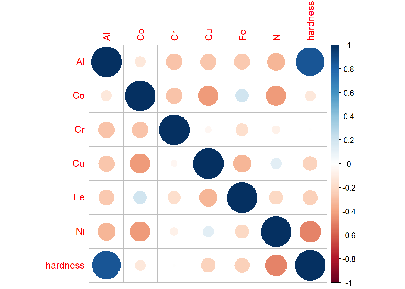
#predict(hard.clr.lm,clr(v))

hard.clr.lm <- lm(y ~ ., cbind(y,hard.clr) %>% data.frame())
hard.ilr.lm <- lm(y ~ ., cbind(y,hard.ilr) %>% data.frame())
hard.alr.lm <- lm(y ~ ., cbind(y,hard.alr) %>% data.frame())
hard.ilr.glm.model <- cv.glmnet(hard.ilr, y, alpha = 1)
hard.ilr.glm <- glmnet(hard.ilr, y, alpha = 1, lambda = hard.ilr.glm.model$lambda.min)dataset <- cbind(data.frame(hardness = y),hard.clr) %>% data.frame()
hard.clr.gam <- gam(hardness ~ Al+ Co + Co + Cr + Cu + Fe + Ni, data = dataset)predictions.full <- data.frame(hard_) %>%
mutate(prediction.clr.lm = predict(hard.clr.lm, newx = hard_),
prediction.ilr.lm = predict(hard.ilr.lm, newx = hard.ilr),
#prediction.alr.lm = predict(hard.alr.lm, newx = hard.alr),
prediction.ilr.glm = predict(hard.ilr.glm, best_lambda = hard.ilr.glm.model$lambda.min, newx = hard.ilr),
prediction.clr.gam = predict(hard.clr.gam, newx = hard.clr),
pre = predict(hard.clr.lm, newx = row()))# predictions.full %>% colnames
predictions.full %>%
arrange(hardness) %>%
mutate(row_name = row_number()) %>%
pivot_longer(c(hardness, prediction.clr.lm,prediction.ilr.glm, prediction.clr.gam), names_to = "variable",values_to = "value") %>%
ggplot(aes(row_name, value, colour = variable, shape = variable))+
geom_point(alpha = 0.8)+
labs(title = "Hardness prediction",
subtitle = "Comparing hardness prediction.clr.lm and actual hardness",
y = "hardness",
x = "rank ordered by ascending hardness")+
#annotate("text", y = 200, x = 25,label = paste("RMSE = ",
# round(RMSE(predictions.full$prediction.clr.lm, predictions.full$hardness),2)
#))+
theme_bw()+
theme(legend.position = c(0.8,0.2),
legend.background = element_rect(fill = "white", color = "black"))+
scale_color_discrete(name = paste("RMSE = ", round(RMSE(predictions.full$prediction.clr.lm, predictions.full$hardness),2)))+
scale_shape_discrete(name = paste("RMSE = ", round(RMSE(predictions.full$prediction.clr.lm, predictions.full$hardness),2)))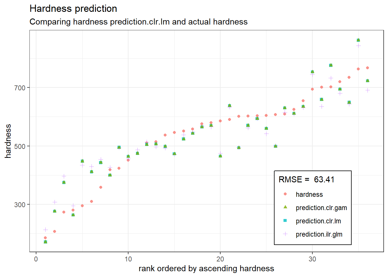
# Linear regression on ILR logratio transformation
RMSE(predictions.full$prediction.clr.lm, predictions.full$hardness)
## [1] 63.40838# Lasso regression on ILR logratio transformation
RMSE(predictions.full$prediction.ilr.glm, predictions.full$hardness)## [1] 65.79862# generalised additive model
RMSE(predictions.full$prediction.clr.gam, predictions.full$hardness)## [1] 63.40838# library(robCompositions)
# aDist(x = hard_[,1:ncol(hard)-1])
#Compositional::alfa.ridge(as.matrix(y), as.matrix(x),a = 0.01, lambda = 1)Principal component analysis for compositional data vectors
Artificial Neural Network (ANN) approach
scale01 <- function(x){
  (x - min(x)) / (max(x) - min(x))
}


scale02 <- function(y){
  y * (max(hard_$hardness) - min(hard_$hardness)) + min(hard_$hardness)
}

scale03 <- function(i){
  i * (max(i) - min(i)) + min(i)
}

hard_ann <- cbind(hard_$hardness,as_tibble(hard.clr)) %>%
  mutate_all(scale01) %>% rename("hardness" = "hard_$hardness")

set.seed(1)
hard_ann_train <- sample_frac(tbl = hard_ann, replace = FALSE, size = 0.80)
hard_ann_test <- anti_join(hard_ann, hard_ann_train)
hard_ann_model1 <- neuralnet(hardness ~ Al + Co +
Cr + Cu + Fe +
Ni, data = hard_ann_train)hard_ann_model2 <- neuralnet(hardness ~ Al + Co +
Cr + Cu + Fe +
Ni, data = hard_ann_train,
hidden = c(4, 1),
act.fct = 'logistic',
rep = 10)hard_ann_test_output1 <- compute(hard_ann_model1, hard_ann_test[, 2:7])$net.result
hard_ann_test_output2 <- compute(hard_ann_model2, hard_ann_test[, 2:7])$net.result
hard_ann_sse1 <- sum((hard_ann_test_output1 - hard_ann_test[, 1])^2)/2
hard_ann_sse2 <- sum((hard_ann_test_output2 - hard_ann_test[, 1])^2)/2
hard_ann_sse1## [1] 0.01869546hard_ann_sse2 # model 2 is more accurate## [1] 0.01810635dat <- cbind(p = hard_ann_test_output2, hard_ann_test) %>%
arrange(hardness) %>%
mutate(row = row_number()) %>%
mutate(prediction = scale02(p),
hardness = scale02(hardness))
dat %>%
pivot_longer(c("prediction","hardness")) %>%
mutate(row = as.integer((row_number()-1)/2)) %>%
ggplot(aes(row, value, colour = name, shape = name)) +
geom_point()+
scale_color_discrete(name = paste("RMSE = ", round(RMSE(dat$prediction,dat$hardness),2)))+
scale_shape_discrete(name = paste("RMSE = ", round(RMSE(dat$prediction,dat$hardness),2)))+
labs(title = "Unseen data observations ANN",
subtitle = "Comparing hardness artificial neural network regression and actual hardness on unseen data")+
theme_bw()+
theme(legend.position = c(0.8,0.2),
legend.background = element_rect(fill = "white", color = "black"))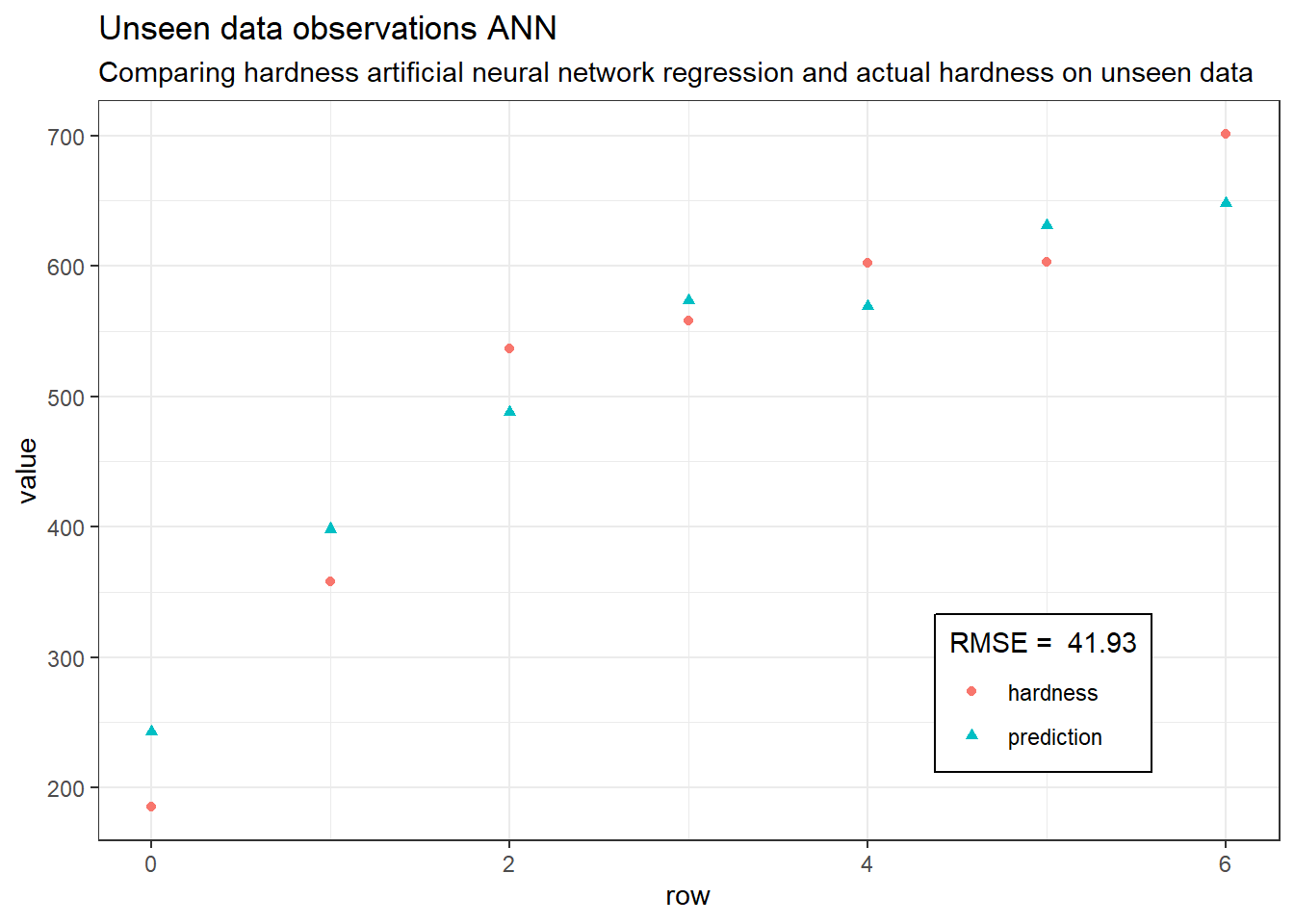
hard_ann_results <- compute(hard_ann_model2, hard_ann[, 2:7])$net.resultdat1 <- cbind(predictions = hard_ann_results, hard_ann) %>%
mutate("ANN prediction" = scale02(predictions),
hardness = scale02(hardness),
distance = `ANN prediction` - hardness) %>%
arrange(hardness)
dat2 <- dat1 %>%
pivot_longer(c("ANN prediction","hardness"), values_to = "val", names_to = "var") %>%
mutate(row = as.integer((row_number()-1)/2))g <- cbind(data.frame(p = hard_ann_results) %>% mutate(p = scale02(p)),hard_ann) %>%
mutate(hardness = scale02(hardness))dat2 %>%
ggplot(aes(row, val, shape = var, colour = var)) +
geom_point()+
scale_color_discrete(type = c("dodgerblue", "red"),name = paste("RMSE = ",round(RMSE(g$p, g$hardness),2)))+
scale_shape_discrete(name = paste("RMSE = ",round(RMSE(g$p, g$hardness),2)))+
labs(title = "Hardness prediction",
subtitle = "Comparing hardness artificial neural network regression and actual hardness",
y = "HV hardness",
x = "rank ordered by ascending hardness")+
#annotate("text", y = 200, x = 25,label = paste("RMSE = ",
# round(RMSE(hard$hardness, dat$predictions),2)
#))+
theme_bw()+
theme(legend.position = c(0.8,0.2),
legend.background = element_rect(fill = "white", color = "black"))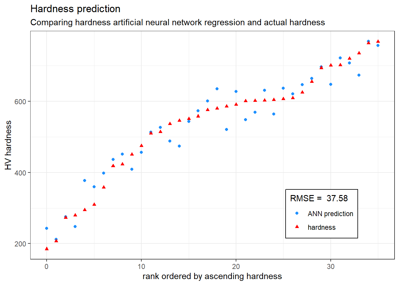
Exploring the compositional space
g <- hard_ann %>%
  arrange(desc(hardness)) %>%
  filter(hardness > 0.8) %>%
  pivot_longer(cols = colnames(hard_ann)[2:7])


#scale04("Co")
#lapply


g %>%
  ggplot(aes(hardness, value, colour = name))+
  geom_line(size = 2)+
  theme_classic()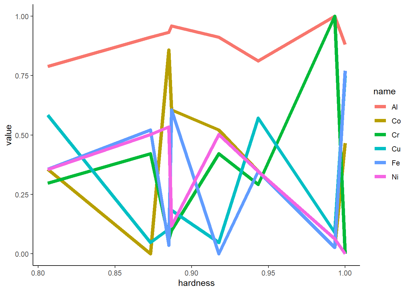
g <- cbind(predictions = hard_ann_results, hard_ann) %>%
  mutate(
    predictions = predictions * (max(hard_$hardness) - min(hard_$hardness)) + min(hard_$hardness),
    hardness = hardness * (max(hard_$hardness) - min(hard_$hardness)) + min(hard_$hardness),
    Al = Al * (max(hard_$Al) - min(hard_$Al)) + min(hard_$Al),
    Co = Co * (max(hard_$Co) - min(hard_$Co)) + min(hard_$Co),
    Cr = Cr * (max(hard_$Cr) - min(hard_$Cr)) + min(hard_$Cr),
    Cu = Cu * (max(hard_$Cu) - min(hard_$Cu)) + min(hard_$Cu),
    Fe = Fe * (max(hard_$Fe) - min(hard_$Fe)) + min(hard_$Fe),
    Ni = Ni * (max(hard_$Ni) - min(hard_$Ni)) + min(hard_$Ni)
  )

hard_ %>% arrange(desc(hardness))
## # A tibble: 36 x 7
## Al Co Cr Cu Fe Ni hardness
## <dbl> <dbl> <dbl> <dbl> <dbl> <dbl> <dbl>
## 1 40 13.3 6.7 13.3 20 6.7 768
## 2 43 6 33 6 6 6 764
## 3 37.5 12.5 12.5 12.5 12.5 12.5 735
## 4 42.9 14.3 14.3 7.1 7.1 14.3 720
## 5 46.2 15.4 7.7 7.7 15.4 7.7 702
## 6 42.9 21.4 7.1 7.1 7.1 14.3 701
## 7 42.9 7.1 14.3 7.1 14.3 14.3 694
## 8 35.9 12.8 12.8 12.8 12.8 12.8 655
## 9 33.3 13.3 13.3 13.3 13.3 13.3 625
## 10 30.8 15.4 15.4 7.7 15.4 15.4 609
## # ... with 26 more rowshard %>% mutate(sum3 = Al + Co + Cr) %>%
ggplot(aes(sum3, hardness))+
geom_line()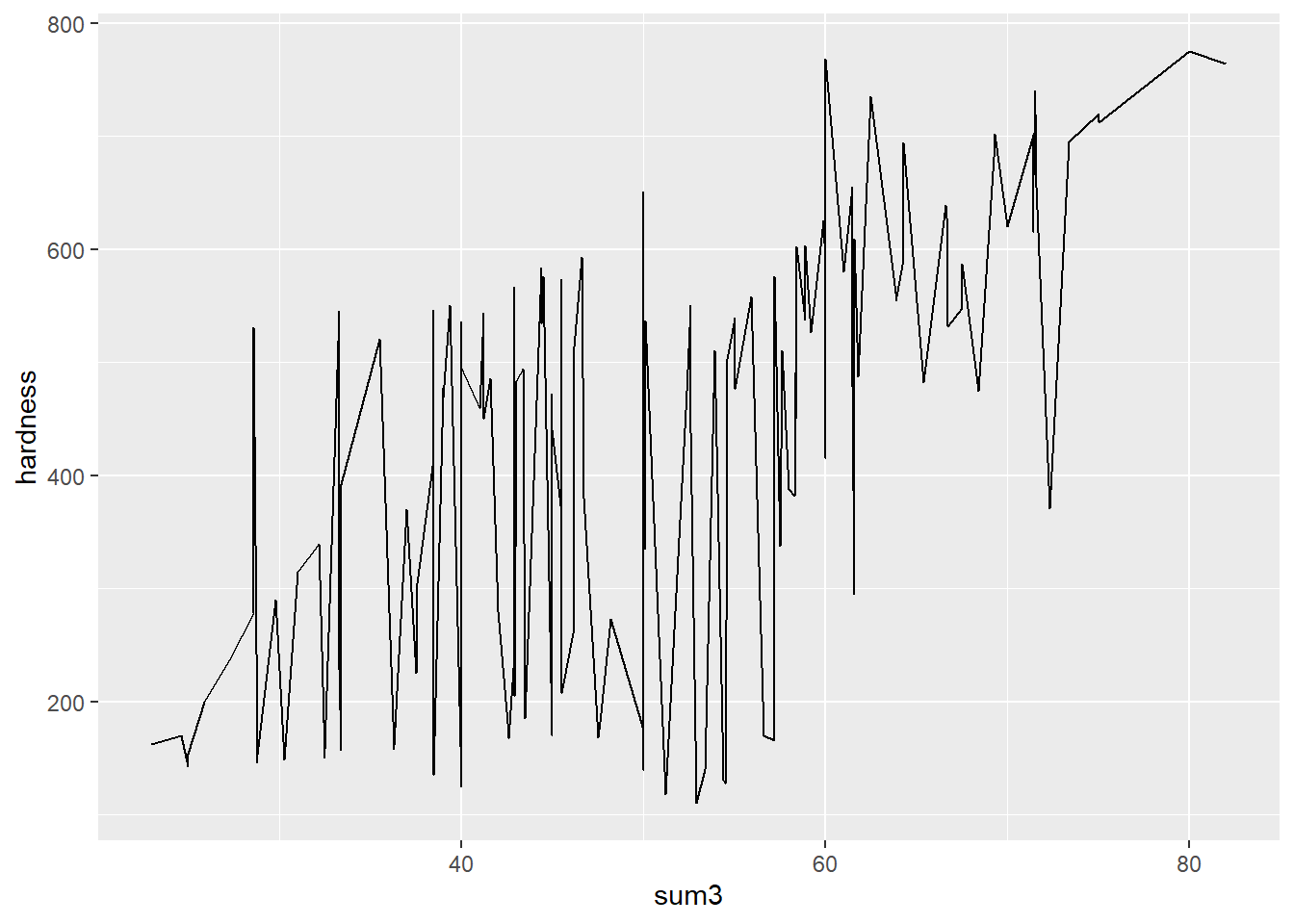
g %>% filter(hardness>650) %>% # high copper, low nickel, cobalt good/midrange, iron good
  ggplot(aes(hardness, colour = Fe))+
  geom_point(aes(y=Al))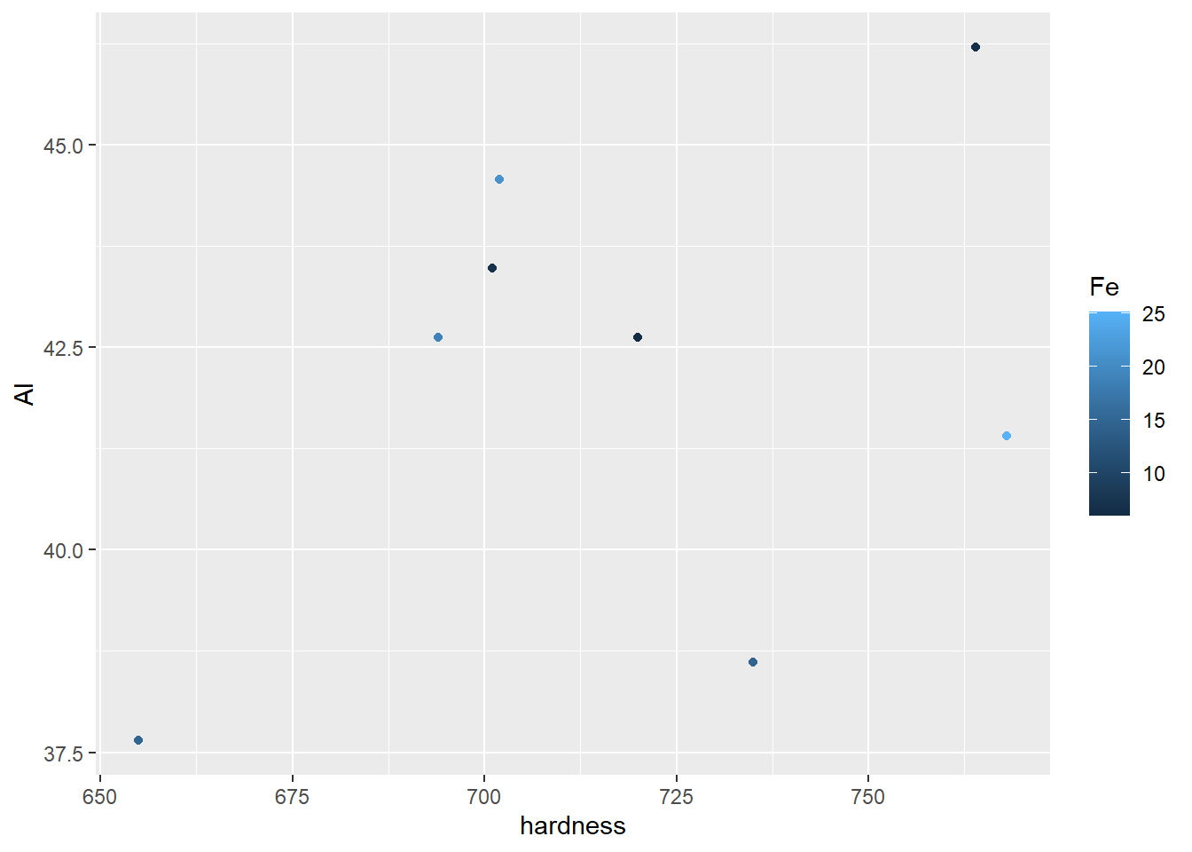
p <- g %>%
  mutate(unseen = 0) %>%
  add_row(predictions = 0, hardness = 0,Al = 40, Co = 20, Cr = 20, Cu = 0, Fe = 20, Ni = 0, unseen = 1) %>%
  add_row(predictions = 0, hardness = 0,Al = 41, Co = 19, Cr = 20, Cu = 0, Fe = 20, Ni = 0, unseen = 1) %>%
  add_row(predictions = 0, hardness = 0,Al = 42, Co = 18, Cr = 20, Cu = 0, Fe = 20, Ni = 0, unseen = 1) %>%
  add_row(predictions = 0, hardness = 0,Al = 41, Co = 20, Cr = 19, Cu = 0, Fe = 20, Ni = 0, unseen = 1) %>%
  add_row(predictions = 0, hardness = 0,Al = 42, Co = 20, Cr = 18, Cu = 0, Fe = 20, Ni = 0, unseen = 1) %>%
  add_row(predictions = 0, hardness = 0,Al = 41, Co = 20, Cr = 20, Cu = 0, Fe = 19, Ni = 0, unseen = 1) %>%
  add_row(predictions = 0, hardness = 0,Al = 42, Co = 20, Cr = 20, Cu = 0, Fe = 18, Ni = 0, unseen = 1) %>%
    add_row(predictions = 0, hardness = 0,Al = 43, Co = 17, Cr = 20, Cu = 0, Fe = 20, Ni = 0, unseen = 1) %>%
    add_row(predictions = 0, hardness = 0,Al = 44, Co = 16, Cr = 20, Cu = 0, Fe = 20, Ni = 0, unseen = 1) %>%
    add_row(predictions = 0, hardness = 0,Al = 45, Co = 15, Cr = 20, Cu = 0, Fe = 20, Ni = 0, unseen = 1) %>%
    add_row(predictions = 0, hardness = 0,Al = 46, Co = 18, Cr = 18, Cu = 0, Fe = 18, Ni = 0, unseen = 1) %>%
    add_row(predictions = 0, hardness = 0,Al = 43, Co = 19, Cr = 19, Cu = 0, Fe = 19, Ni = 0, unseen = 1) %>%
  add_row(predictions = 0, hardness = 0,Al = 49, Co = 17, Cr = 17, Cu = 0, Fe = 17, Ni = 0, unseen = 1) %>%
  add_row(predictions = 0, hardness = 0,Al = 30:50, Co = 30:10, Cr = 20, Cu = 0, Fe = 20, Ni = 0, unseen = 1) %>%
  add_row(predictions = 0, hardness = 0,Al = 30:50, Co = 20, Cr = 30:10, Cu = 0, Fe = 20, Ni = 0, unseen = 1) %>%
  add_row(predictions = 0, hardness = 0,Al = 30:50, Co = 20, Cr = 20, Cu = 0, Fe = 30:10, Ni = 0, unseen = 1) %>%
  add_row(predictions = 0, hardness = 0,Al = 20:60, Co = 40:0, Cr = 20, Cu = 0, Fe = 20, Ni = 0, unseen = 1)


predictions <- compute(hard_ann_model2, p[, 3:8])$net.result

t <- cbind(predictions,p[,2:9]) %>%
    mutate(
    predictions = predictions * (max(hard_$hardness) - min(hard_$hardness)) + min(hard_$hardness)) %>%
  distinct()


t_plot <- t %>% arrange(predictions) %>%
  mutate(rank = row_number()) %>%
  mutate(composition = paste("Al",round(Al),"Co",round(Co),"Cr",round(Cr),"Cu",round(Cu),"Fe",round(Fe),"Ni",round(Ni))) %>%
  ggplot(aes(rank, predictions, colour = as.factor(unseen), shape = as.factor(unseen), group = composition))+
  geom_point()+
  scale_color_discrete(type = c("red", "dodgerblue"),name = "unseen")+
  scale_shape_discrete(name = "unseen")+
  labs(title = "Hardness prediction in a virtual space",
       subtitle = "Exploring a virtual compositional space with the ANN model",
       y = "HV hardness",
       x = "rank ordered by ascending hardness")+
  #annotate("text", y = 200, x = 25,label = paste("RMSE = ",
  #  round(RMSE(hard$hardness, dat$predictions),2)
  #))+
  theme_bw()+
  theme(legend.position = c(0.8,0.2),
        legend.background = element_rect(fill = "white", color = "black"))

plotly::ggplotly(t_plot)
hard %>% filter(Co<15,Al>40) %>%
arrange(desc(hardness))## # A tibble: 5 x 7
## Al Co Cr Cu Fe Ni hardness
## <dbl> <dbl> <dbl> <dbl> <dbl> <dbl> <dbl>
## 1 43 6 33 6 6 6 764
## 2 42.9 14.3 14.3 0 14.3 14.3 740
## 3 42.9 14.3 14.3 7.1 7.1 14.3 720
## 4 42.9 7.1 14.3 7.1 14.3 14.3 694
## 5 42.9 14.3 7.1 7.1 7.1 21.4 591