Election2019

Voting mix of the most populated constituencies

party_colours <- c("purple", "dodgerblue", "red","orange","yellow")
election %>% 
  arrange(desc(valid_votes)) %>% 
  mutate(constituency_name=fct_reorder(constituency_name,con_p)) %>% 
  head(30) %>% 
  gather(key="Party", value="Number", con, lab, ld, snp, brexit) %>% 
  ggplot(aes(constituency_name,Number,fill=Party))+
  geom_col()+
  scale_fill_manual(values=party_colours)+
  coord_flip()+
  bbc_style()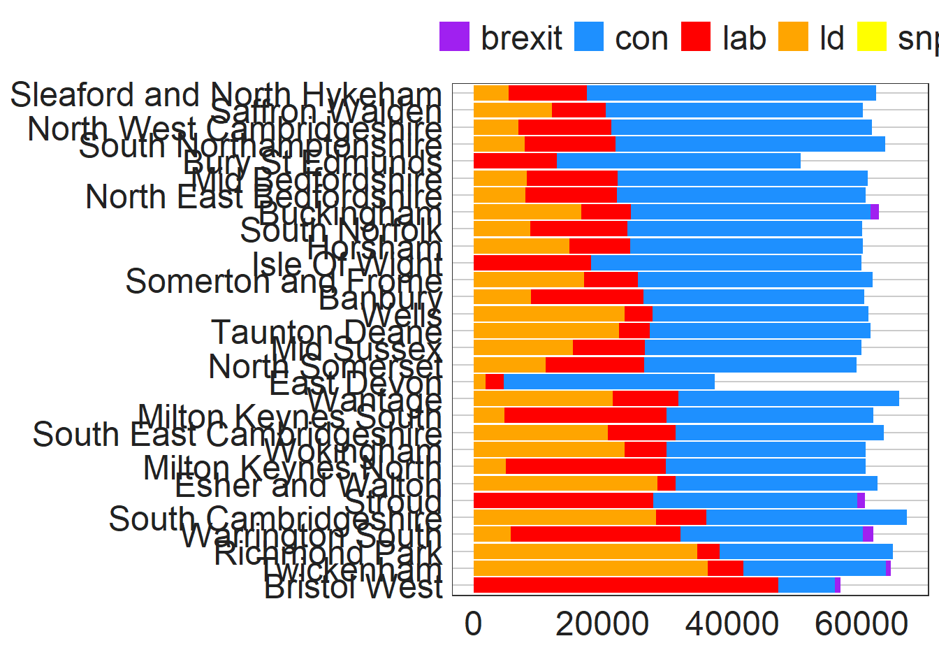

Voting mix of the least populated constituencies

election %>% 
  arrange(valid_votes) %>% 
  mutate(constituency_name=fct_reorder(constituency_name,valid_votes)) %>% 
  head(30) %>% 
  gather(key="Party", value="Number", con, lab, ld, snp, brexit) %>% 
  ggplot(aes(constituency_name,Number,fill=Party))+
  geom_col()+
  scale_fill_manual(values=party_colours)+
  coord_flip()+
  bbc_style()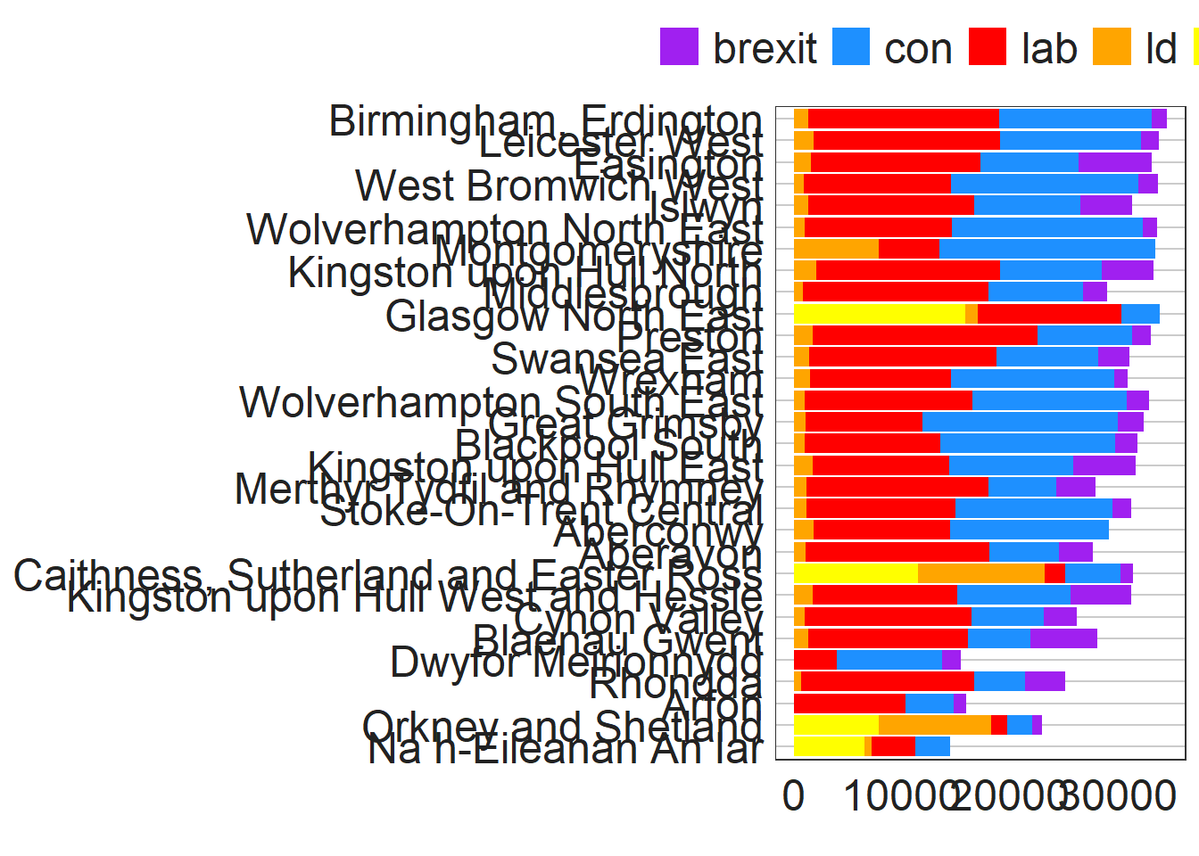

Where are the Conservative strongholds?

election %>% 
  arrange(desc(con_p)) %>% 
  mutate(constituency_name=fct_reorder(constituency_name,con_p)) %>% 
  head(30) %>%
  gather(Party, Proportion, con_p, lab_p, ld_p, brexit_p, snp_p) %>% 
  ggplot(aes(constituency_name,Proportion, fill = Party))+
  geom_col()+
  scale_fill_manual(values=party_colours)+
  scale_y_continuous(label=scales::percent_format()) +
  coord_flip()+
  bbc_style()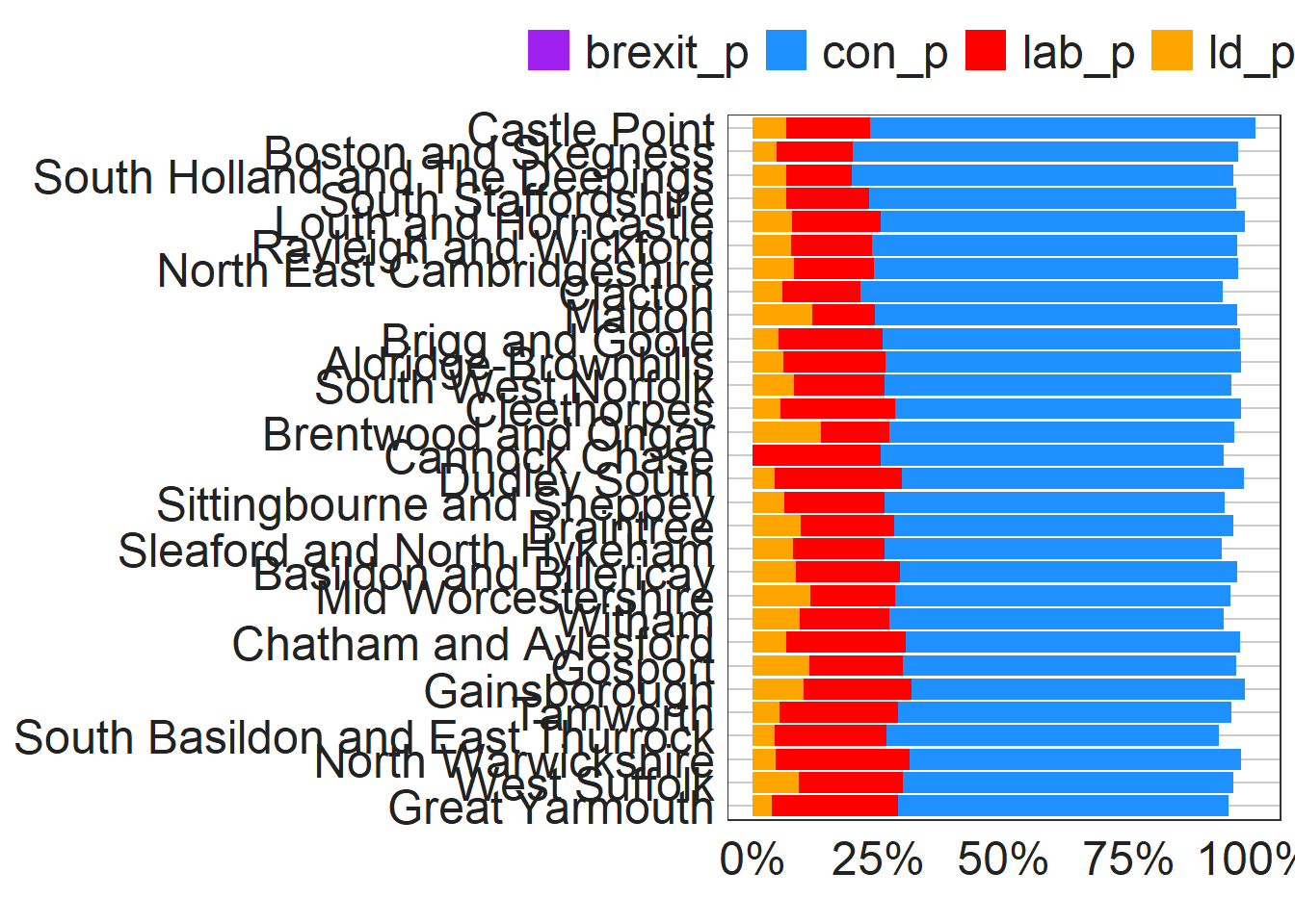

Brexit Party significance

election %>% 
  mutate(constituency_name=fct_reorder(constituency_name, -con_p)) %>% 
  arrange(con_p) %>% 
  gather(Party, Proportion, con_p, lab_p, snp_p, brexit_p, ld_p) %>% 
  ggplot(aes(constituency_name, Proportion, fill = Party)) +
  geom_col()+
  scale_fill_manual(values=party_colours)+
  scale_x_discrete(expand = c(0,0))+
  scale_y_continuous(expand = c(0,0))+
  labs(
    x="",
    y="Vote Share"
  )+
 bbc_style()+
  theme(axis.text.x = element_blank())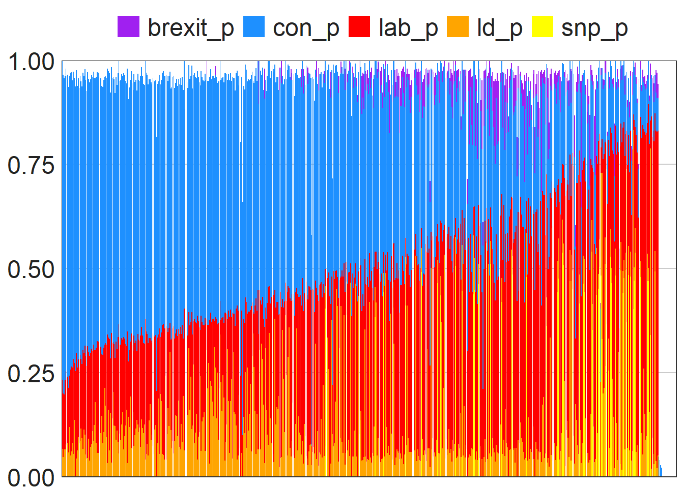

election %>% 
  ggplot(aes(con_p)) +
  geom_histogram(fill=party_colours[2])+
  bbc_style()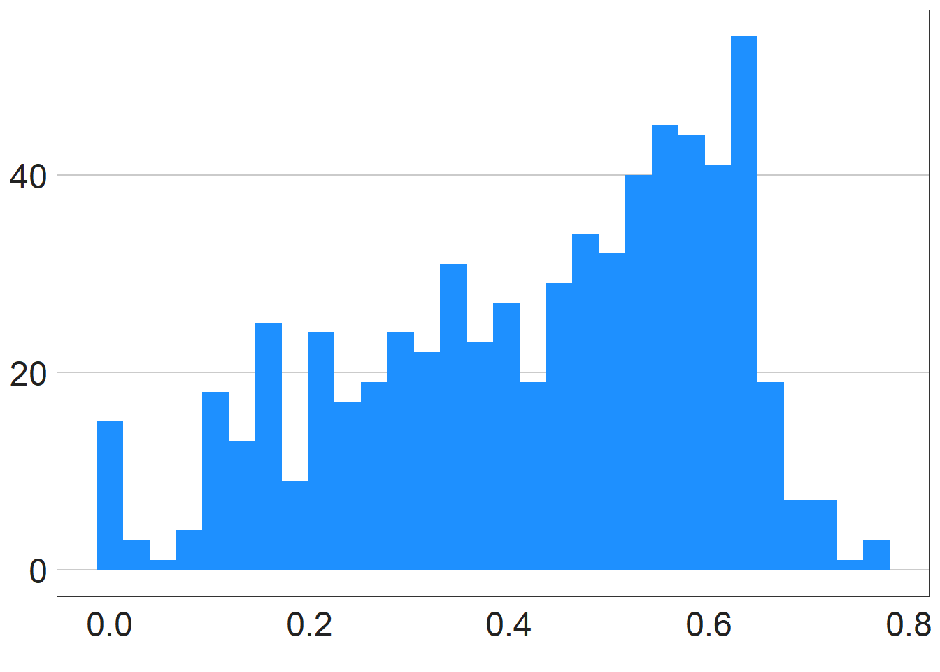

election %>% 
  ggplot(aes(lab_p))+
  geom_histogram(fill=party_colours[3])+
  bbc_style()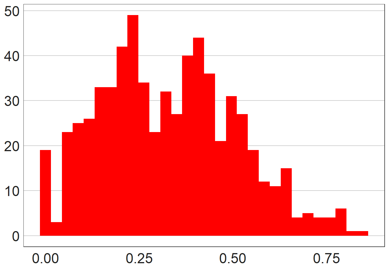

election %>% 
  ggplot(aes(brexit_p))+
  geom_histogram(fill=party_colours[1])+
  bbc_style()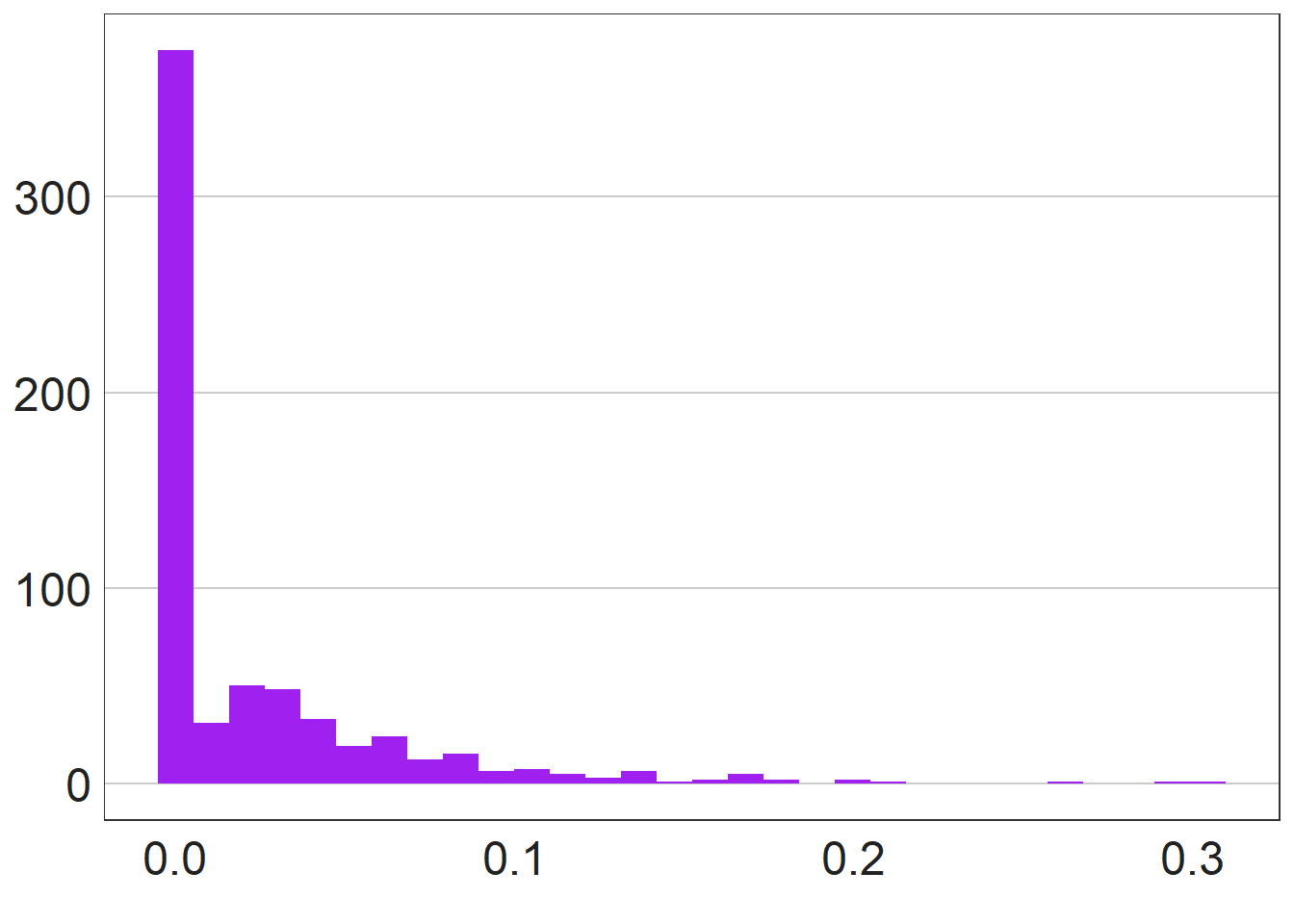

election %>%
  filter(!brexit_p==0) %>% 
  ggplot(aes(brexit_p))+
  geom_histogram(fill=party_colours[1])+
  bbc_style()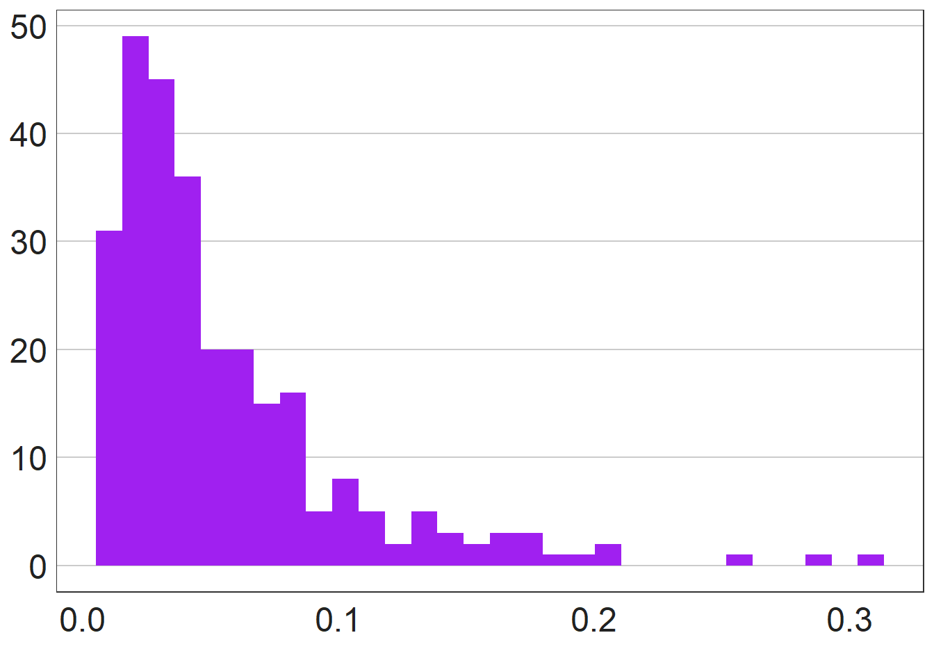

election_noscotland <- election %>% 
  filter(!country_name=="Scotland")
  
model.lm <- lm(brexit_p ~ con_p + lab_p + ld_p, data = election_noscotland)
library(broom)
tidy(model.lm)

## # A tibble: 4 x 5
##   term        estimate std.error statistic  p.value
##   <chr>          <dbl>     <dbl>     <dbl>    <dbl>
## 1 (Intercept)   0.0464   0.00802      5.78 1.19e- 8
## 2 con_p        -0.0651   0.0104      -6.29 6.36e-10
## 3 lab_p         0.0436   0.0109       3.99 7.58e- 5
## 4 ld_p         -0.0661   0.0170      -3.88 1.16e- 4

election_wales <- election %>% 
  filter(country_name=="Wales")
model.lm <- lm(brexit_p ~ con_p + lab_p + ld_p, data = election_wales)
tidy(model.lm)

## # A tibble: 4 x 5
##   term         estimate std.error statistic   p.value
##   <chr>           <dbl>     <dbl>     <dbl>     <dbl>
## 1 (Intercept)  0.157       0.0369   4.26    0.000140 
## 2 con_p       -0.264       0.0547  -4.82    0.0000261
## 3 lab_p        0.000206    0.0563   0.00365 0.997    
## 4 ld_p        -0.104       0.0926  -1.12    0.271

Significant evidence shows that the participation of the Brexit Party in the election tends to reduce the Conservative vote share. Conversely, as the Brexit Party vote share increases, the Labour vote share increases by a small amount. This may suggest that the selective nature of the Brexit Party choosing which seats to contest has aided the Conservatives in the FPTP system.